1.5 Basic Data Manipulation
The learning objectives for this section are to:
- Transform non-tidy data into tidy data
- Manipulate and transform a variety of data types, including dates, times, and text data
The two packages dplyr and tidyr, both “tidyverse” packages, allow you to quickly and fairly easily clean up your data. These packages are not very old, and so much of the example R code you might find in books or online might not use the functions we use in examples in this section (although this is quickly changing for new books and for online examples). Further, there are many people who are used to using R base functionality to clean up their data, and some of them still do not use these packages much when cleaning data. We think, however, that dplyr is easier for people new to R to learn than learning how to clean up data using base R functions, and we also think it produces code that is much easier to read, which is useful in maintaining and sharing code.
For many of the examples in this section, we will use the ext_tracks hurricane dataset we input from a url as an example in a previous section of this book. If you need to load a version of that data, we have also saved it locally, so you can create an R object with the example data for this section by running:
ext_tracks_file <- "data/ebtrk_atlc_1988_2015.txt"
ext_tracks_widths <- c(7, 10, 2, 2, 3, 5, 5, 6, 4, 5, 4, 4, 5, 3, 4, 3, 3, 3,
                       4, 3, 3, 3, 4, 3, 3, 3, 2, 6, 1)
ext_tracks_colnames <- c("storm_id", "storm_name", "month", "day",
                          "hour", "year", "latitude", "longitude",
                          "max_wind", "min_pressure", "rad_max_wind",
                          "eye_diameter", "pressure_1", "pressure_2",
                          paste("radius_34", c("ne", "se", "sw", "nw"), sep = "_"),
                          paste("radius_50", c("ne", "se", "sw", "nw"), sep = "_"),
                          paste("radius_64", c("ne", "se", "sw", "nw"), sep = "_"),
                          "storm_type", "distance_to_land", "final")
ext_tracks <- read_fwf(ext_tracks_file,
                       fwf_widths(ext_tracks_widths, ext_tracks_colnames),
                       na = "-99")
1.5.1 Piping
The dplyr and tidyr functions are often used in conjunction with piping, which is done with the %>% function from the magrittr package. Piping can be done with many R functions, but is especially common with dplyr and tidyr functions. The concept is straightforward– the pipe passes the data frame output that results from the function right before the pipe to input it as the first argument of the function right after the pipe.
Here is a generic view of how this works in code, for a pseudo-function named function that inputs a data frame as its first argument:
# Without piping
function(dataframe, argument_2, argument_3)

# With piping
dataframe %>%
  function(argument_2, argument_3)
For example, without piping, if you wanted to see the time, date, and maximum winds for Katrina from the first three rows of the ext_tracks hurricane data, you could run:
katrina <- filter(ext_tracks, storm_name == "KATRINA")
katrina_reduced <- select(katrina, month, day, hour, max_wind)
head(katrina_reduced, 3)
# A tibble: 3 x 4
  month day   hour  max_wind
  <chr> <chr> <chr>    <dbl>
1 10    28    18          30
2 10    29    00          30
3 10    29    06          30
In this code, you are creating new R objects at each step, which makes the code cluttered and also requires copying the data frame several times into memory. As an alternative, you could just wrap one function inside another:
head(select(filter(ext_tracks, storm_name == "KATRINA"),
            month, day, hour, max_wind), 3)
# A tibble: 3 x 4
  month day   hour  max_wind
  <chr> <chr> <chr>    <dbl>
1 10    28    18          30
2 10    29    00          30
3 10    29    06          30
This avoids re-assigning the data frame at each step, but quickly becomes ungainly, and it’s easy to put arguments in the wrong layer of parentheses. Piping avoids these problems, since at each step you can send the output from the last function into the next function as that next function’s first argument:
ext_tracks %>%
  filter(storm_name == "KATRINA") %>%
  select(month, day, hour, max_wind) %>%
  head(3)
# A tibble: 3 x 4
  month day   hour  max_wind
  <chr> <chr> <chr>    <dbl>
1 10    28    18          30
2 10    29    00          30
3 10    29    06          30
1.5.2 Summarizing data
The dplyr and tidyr packages have numerous functions (sometimes referred to as “verbs”) for cleaning up data. We’ll start with the functions to summarize data.
The primary of these is summarize, which inputs a data frame and creates a new data frame with the requested summaries. In conjunction with summarize, you can use other functions from dplyr (e.g., n, which counts the number of observations in a given column) to create this summary. You can also use R functions from other packages or base R functions to create the summary.
For example, say we want a summary of the number of observations in the ext_tracks hurricane dataset, as well as the highest measured maximum windspeed (given by the column max_wind in the dataset) in any of the storms, and the lowest minimum pressure (min_pressure). To create this summary, you can run:
ext_tracks %>%
  summarize(n_obs = n(),
            worst_wind = max(max_wind),
            worst_pressure = min(min_pressure))
# A tibble: 1 x 3
  n_obs worst_wind worst_pressure
  <int>      <dbl>          <dbl>
1 11824        160              0
This summary provides particularly useful information for this example data, because it gives an unrealistic value for minimum pressure (0 hPa). This shows that this dataset will need some cleaning. The highest wind speed observed for any of the storms, 160 knots, is more reasonable.
You can also use summarize with functions you’ve written yourself, which gives you a lot of power in summarizing data in interesting ways. As a simple example, if you wanted to present the maximum wind speed in the summary above using miles per hour rather than knots, you could write a function to perform the conversion, and then use that function within the summarize call:
knots_to_mph <- function(knots){
  mph <- 1.152 * knots
}

ext_tracks %>%
  summarize(n_obs = n(),
            worst_wind = knots_to_mph(max(max_wind)),
            worst_pressure = min(min_pressure))
# A tibble: 1 x 3
  n_obs worst_wind worst_pressure
  <int>      <dbl>          <dbl>
1 11824       184.              0
So far, we’ve only used summarize to create a single-line summary of the data frame. In other words, the summary functions are applied across the entire dataset, to return a single value for each summary statistic. However, often you might want summaries stratified by a certain grouping characteristic of the data. For the hurricane data, for example, you might want to get the worst wind and worst pressure by storm, rather than across all storms.
You can do this by grouping your data frame by one of its column variables, using the function group_by, and then using summarize. The group_by function does not make a visible change to a data frame, although you can see, if you print out a grouped data frame, that the new grouping variable will be listed under “Groups” at the top of a print-out:
ext_tracks %>%
  group_by(storm_name, year) %>%
  head()
# A tibble: 6 x 29
# Groups:   storm_name, year [1]
  storm_id storm_name month day   hour   year latitude longitude max_wind
  <chr>    <chr>      <chr> <chr> <chr> <dbl>    <dbl>     <dbl>    <dbl>
1 AL0188   ALBERTO    08    05    18     1988     32        77.5       20
2 AL0188   ALBERTO    08    06    00     1988     32.8      76.2       20
3 AL0188   ALBERTO    08    06    06     1988     34        75.2       20
4 AL0188   ALBERTO    08    06    12     1988     35.2      74.6       25
5 AL0188   ALBERTO    08    06    18     1988     37        73.5       25
6 AL0188   ALBERTO    08    07    00     1988     38.7      72.4       25
# … with 20 more variables: min_pressure <dbl>, rad_max_wind <dbl>,
#   eye_diameter <dbl>, pressure_1 <dbl>, pressure_2 <dbl>, radius_34_ne <dbl>,
#   radius_34_se <dbl>, radius_34_sw <dbl>, radius_34_nw <dbl>,
#   radius_50_ne <dbl>, radius_50_se <dbl>, radius_50_sw <dbl>,
#   radius_50_nw <dbl>, radius_64_ne <dbl>, radius_64_se <dbl>,
#   radius_64_sw <dbl>, radius_64_nw <dbl>, storm_type <chr>,
#   distance_to_land <dbl>, final <chr>
As a note, since hurricane storm names repeat at regular intervals until they are retired, to get a separate summary for each unique storm, this example requires grouping by both storm_name and year.
Even though applying the group_by function does not cause a noticeable change to the data frame itself, you’ll notice the difference in grouped and ungrouped data frames when you use summarize on the data frame. If a data frame is grouped, all summaries are calculated and given separately for each unique value of the grouping variable:
ext_tracks %>%
  group_by(storm_name, year) %>%
  summarize(n_obs = n(),
            worst_wind = max(max_wind),
            worst_pressure = min(min_pressure))
`summarise()` regrouping output by 'storm_name' (override with `.groups` argument)
# A tibble: 378 x 5
# Groups:   storm_name [160]
   storm_name  year n_obs worst_wind worst_pressure
   <chr>      <dbl> <int>      <dbl>          <dbl>
 1 ALBERTO     1988    13         35           1002
 2 ALBERTO     1994    31         55            993
 3 ALBERTO     2000    87        110            950
 4 ALBERTO     2006    37         60            969
 5 ALBERTO     2012    20         50            995
 6 ALEX        1998    26         45           1002
 7 ALEX        2004    25        105            957
 8 ALEX        2010    30         90            948
 9 ALLISON     1989    28         45            999
10 ALLISON     1995    33         65            982
# … with 368 more rows
This grouping / summarizing combination can be very useful for quickly plotting interesting summaries of a dataset. For example, to plot a histogram of maximum wind speed observed for each storm (Figure 1.1), you could run:
library(ggplot2)
ext_tracks %>%
  group_by(storm_name) %>%
  summarize(worst_wind = max(max_wind)) %>%
ggplot(aes(x = worst_wind)) + geom_histogram() 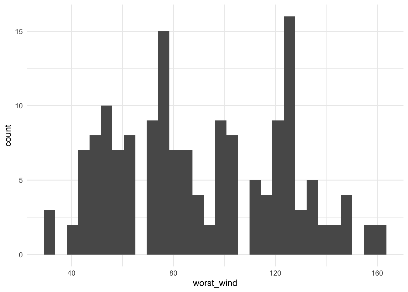
Figure 1.1: Histogram of the maximum wind speed observed during a storm for all Atlantic basin tropical storms, 1988–2015.
A> We will show a few basic examples of plotting using ggplot2 functions in this chapter of the book. We will cover plotting much more thoroughly in a later section of the specialization.
From Figure 1.1, we can see that only two storms had maximum wind speeds at or above 160 knots (we’ll check this later with some other dplyr functions).
T> You cannot make changes to a variable that is being used to group a dataframe. If you try, you will get the error Error: cannot modify grouping variable. If you get this error, use the ungroup function to remove grouping within a data frame, and then you will be able to mutate any of the variables in the data.
1.5.3 Selecting and filtering data
When cleaning up data, you will need to be able to create subsets of the data, by selecting certain columns or filtering down to certain rows. These actions can be done using the dplyr functions select and filter.
The select function subsets certain columns of a data frame. The most basic way to use select is select certain columns by specifying their full column names. For example, to select the storm name, date, time, latitude, longitude, and maximum wind speed from the ext_tracks dataset, you can run:
ext_tracks %>%
  select(storm_name, month, day, hour, year, latitude, longitude, max_wind)
# A tibble: 11,824 x 8
   storm_name month day   hour   year latitude longitude max_wind
   <chr>      <chr> <chr> <chr> <dbl>    <dbl>     <dbl>    <dbl>
 1 ALBERTO    08    05    18     1988     32        77.5       20
 2 ALBERTO    08    06    00     1988     32.8      76.2       20
 3 ALBERTO    08    06    06     1988     34        75.2       20
 4 ALBERTO    08    06    12     1988     35.2      74.6       25
 5 ALBERTO    08    06    18     1988     37        73.5       25
 6 ALBERTO    08    07    00     1988     38.7      72.4       25
 7 ALBERTO    08    07    06     1988     40        70.8       30
 8 ALBERTO    08    07    12     1988     41.5      69         35
 9 ALBERTO    08    07    18     1988     43        67.5       35
10 ALBERTO    08    08    00     1988     45        65.5       35
# … with 11,814 more rows
There are several functions you can use with select that give you more flexibility, and so allow you to select columns without specifying the full names of each column. For example, the starts_with function can be used within a select function to pick out all the columns that start with a certain text string. As an example of using starts_with in conjunction with select, in the ext_tracks hurricane data, there are a number of columns that say how far from the storm center winds of certain speeds extend. Tropical storms often have asymmetrical wind fields, so these wind radii are given for each quadrant of the storm (northeast, southeast, northwest, and southeast of the storm’s center). All of the columns with the radius to which winds of 34 knots or more extend start with “radius_34.” To get a dataset with storm names, location, and radii of winds of 34 knots, you could run:
ext_tracks %>%
  select(storm_name, latitude, longitude, starts_with("radius_34"))
# A tibble: 11,824 x 7
   storm_name latitude longitude radius_34_ne radius_34_se radius_34_sw
   <chr>         <dbl>     <dbl>        <dbl>        <dbl>        <dbl>
 1 ALBERTO        32        77.5            0            0            0
 2 ALBERTO        32.8      76.2            0            0            0
 3 ALBERTO        34        75.2            0            0            0
 4 ALBERTO        35.2      74.6            0            0            0
 5 ALBERTO        37        73.5            0            0            0
 6 ALBERTO        38.7      72.4            0            0            0
 7 ALBERTO        40        70.8            0            0            0
 8 ALBERTO        41.5      69            100          100           50
 9 ALBERTO        43        67.5          100          100           50
10 ALBERTO        45        65.5           NA           NA           NA
# … with 11,814 more rows, and 1 more variable: radius_34_nw <dbl>
Other functions that can be used with select in a similar way include:
ends_with: Select all columns that end with a certain string (for example,select(ext_tracks, ends_with("ne"))to get all the wind radii for the northeast quadrant of a storm for the hurricane example data)contains: Select all columns that include a certain string (select(ext_tracks, contains("34"))to get all wind radii for 34-knot winds)matches: Select all columns that match a certain relative expression (select(ext_tracks, matches("_[0-9][0-9]_"))to get all columns where the column name includes two numbers between two underscores, a pattern that matches all of the wind radii columns)
While select picks out certain columns of the data frame, filter picks out certain rows. With filter, you can specify certain conditions using R’s logical operators, and the function will return rows that meet those conditions.
R’s logical operators include:
| Operator | Meaning | Example |
|---|---|---|
== |
Equals | storm_name == KATRINA |
!= |
Does not equal | min_pressure != 0 |
> |
Greater than | latitude > 25 |
>= |
Greater than or equal to | max_wind >= 160 |
< |
Less than | min_pressure < 900 |
<= |
Less than or equal to | distance_to_land <= 0 |
%in% |
Included in | storm_name %in% c("KATRINA", "ANDREW") |
is.na() |
Is a missing value | is.na(radius_34_ne) |
If you are ever unsure of how to write a logical statement, but know how to write its opposite, you can use the ! operator to negate the whole statement. For example, if you wanted to get all storms except those named “KATRINA” and “ANDREW,” you could use !(storm_name %in% c("KATRINA", "ANDREW")). A common use of this is to identify observations with non-missing data (e.g., !(is.na(radius_34_ne))).
A logical statement, run by itself on a vector, will return a vector of the same length with TRUE every time the condition is met and FALSE every time it is not.
head(ext_tracks$hour)
[1] "18" "00" "06" "12" "18" "00"
head(ext_tracks$hour == "00")
[1] FALSE  TRUE FALSE FALSE FALSE  TRUE
When you use a logical statement within filter, it will return just the rows where the logical statement is true:
ext_tracks %>%
  select(storm_name, hour, max_wind) %>%
  head(9)
# A tibble: 9 x 3
  storm_name hour  max_wind
  <chr>      <chr>    <dbl>
1 ALBERTO    18          20
2 ALBERTO    00          20
3 ALBERTO    06          20
4 ALBERTO    12          25
5 ALBERTO    18          25
6 ALBERTO    00          25
7 ALBERTO    06          30
8 ALBERTO    12          35
9 ALBERTO    18          35

ext_tracks %>%
  select(storm_name, hour, max_wind) %>%
  filter(hour == "00") %>%
  head(3)
# A tibble: 3 x 3
  storm_name hour  max_wind
  <chr>      <chr>    <dbl>
1 ALBERTO    00          20
2 ALBERTO    00          25
3 ALBERTO    00          35
Filtering can also be done after summarizing data. For example, to determine which storms had maximum wind speed equal to or above 160 knots, run:
ext_tracks %>%
  group_by(storm_name, year) %>%
  summarize(worst_wind = max(max_wind)) %>%
  filter(worst_wind >= 160)
`summarise()` regrouping output by 'storm_name' (override with `.groups` argument)
# A tibble: 2 x 3
# Groups:   storm_name [2]
  storm_name  year worst_wind
  <chr>      <dbl>      <dbl>
1 GILBERT     1988        160
2 WILMA       2005        160
If you would like to string several logical conditions together and select rows where all or any of the conditions are true, you can use the “and” (&) or “or” (|) operators. For example, to pull out observations for Hurricane Andrew when it was at or above Category 5 strength (137 knots or higher), you could run:
ext_tracks %>%
  select(storm_name, month, day, hour, latitude, longitude, max_wind) %>%
  filter(storm_name == "ANDREW" & max_wind >= 137)
# A tibble: 2 x 7
  storm_name month day   hour  latitude longitude max_wind
  <chr>      <chr> <chr> <chr>    <dbl>     <dbl>    <dbl>
1 ANDREW     08    23    12        25.4      74.2      145
2 ANDREW     08    23    18        25.4      75.8      150
W> Some common errors that come up when using logical operators in R are:
W>
W> - If you want to check that two things are equal, make sure you use double equal signs (==), not a single one. At best, a single equals sign won’t work; in some cases, it will cause a variable to be re-assigned (= can be used for assignment, just like <-).
W> - If you are trying to check if one thing is equal to one of several things, use %in% rather than ==. For example, if you want to filter to rows of ext_tracks with storm names of “KATRINA” and “ANDREW,” you need to use storm_name %in% c("KATRINA", "ANDREW"), not storm_name == c("KATRINA", "ANDREW").
W> - If you want to identify observations with missing values (or without missing values), you must use the is.na function, not == or !=. For example, is.na(radius_34_ne) will work, but radius_34_ne == NA will not.
1.5.4 Adding, changing, or renaming columns
The mutate function in dplyr can be used to add new columns to a data frame or change existing columns in the data frame. As an example, I’ll use the worldcup dataset from the package faraway, which statistics from the 2010 World Cup. To load this example data frame, you can run:
library(faraway)
data(worldcup)
This dataset has observations by player, including the player’s team, position, amount of time played in this World Cup, and number of shots, passes, tackles, and saves. This dataset is currently not tidy, as it has one of the variables (players’ names) as rownames, rather than as a column of the data frame. You can use the mutate function to move the player names to its own column:
worldcup <- worldcup %>%
  mutate(player_name = rownames(worldcup))

worldcup %>% slice(1:3)
     Team   Position Time Shots Passes Tackles Saves player_name
1 Algeria Midfielder   16     0      6       0     0      Abdoun
2   Japan Midfielder  351     0    101      14     0         Abe
3  France   Defender  180     0     91       6     0      Abidal
You can also use mutate in coordination with group_by to create new columns that give summaries within certain windows of the data. For example, the following code will add a column with the average number of shots for a player’s position added as a new column. While this code is summarizing the original data to generate the values in this column, mutate will add these repeated summary values to the original dataset by group, rather than returning a dataframe with a single row for each of the grouping variables (try replacing mutate with summarize in this code to make sure you understand the difference).
worldcup <- worldcup %>%
  group_by(Position) %>%
  mutate(ave_shots = mean(Shots)) %>%
  ungroup()

worldcup %>% slice(1:3)
# A tibble: 3 x 9
  Team    Position    Time Shots Passes Tackles Saves player_name ave_shots
  <fct>   <fct>      <int> <int>  <int>   <int> <int> <chr>           <dbl>
1 Algeria Midfielder    16     0      6       0     0 Abdoun           2.39
2 Japan   Midfielder   351     0    101      14     0 Abe              2.39
3 France  Defender     180     0     91       6     0 Abidal           1.16
If there is a column that you want to rename, but not change, you can use the rename function. For example:
worldcup %>%
  rename(Name = player_name) %>%
  slice(1:3)
# A tibble: 3 x 9
  Team    Position    Time Shots Passes Tackles Saves Name   ave_shots
  <fct>   <fct>      <int> <int>  <int>   <int> <int> <chr>      <dbl>
1 Algeria Midfielder    16     0      6       0     0 Abdoun      2.39
2 Japan   Midfielder   351     0    101      14     0 Abe         2.39
3 France  Defender     180     0     91       6     0 Abidal      1.16
1.5.5 Spreading and gathering data
The tidyr package includes functions to transfer a data frame between long and wide. Wide format data tends to have different attributes or variables describing an observation placed in separate columns. Long format data tends to have different attributes encoded as levels of a single variable, followed by another column that contains tha values of the observation at those different levels.
In the section on tidy data, we showed an example that used gather to convert data into a tidy format. The data is first in an untidy format:
data("VADeaths")
head(VADeaths)
      Rural Male Rural Female Urban Male Urban Female
50-54       11.7          8.7       15.4          8.4
55-59       18.1         11.7       24.3         13.6
60-64       26.9         20.3       37.0         19.3
65-69       41.0         30.9       54.6         35.1
70-74       66.0         54.3       71.1         50.0
After changing the age categories from row names to a variable (which can be done with the mutate function), the key problem with the tidyness of the data is that the variables of urban / rural and male / female are not in their own columns, but rather are embedded in the structure of the columns. To fix this, you can use the gather function to gather values spread across several columns into a single column, with the column names gathered into a “key” column. When gathering, exclude any columns that you don’t want “gathered” (age in this case) by including the column names with a the minus sign in the gather function. For example:
data("VADeaths")
library(tidyr)

# Move age from row names into a column
VADeaths  <- VADeaths %>%
  tbl_df() %>%
  mutate(age = row.names(VADeaths))
VADeaths
# A tibble: 5 x 5
  `Rural Male` `Rural Female` `Urban Male` `Urban Female` age
         <dbl>          <dbl>        <dbl>          <dbl> <chr>
1         11.7            8.7         15.4            8.4 50-54
2         18.1           11.7         24.3           13.6 55-59
3         26.9           20.3         37             19.3 60-64
4         41             30.9         54.6           35.1 65-69
5         66             54.3         71.1           50   70-74

# Gather everything but age to tidy data
VADeaths %>%
  gather(key = key, value = death_rate, -age)
# A tibble: 20 x 3
   age   key          death_rate
   <chr> <chr>             <dbl>
 1 50-54 Rural Male         11.7
 2 55-59 Rural Male         18.1
 3 60-64 Rural Male         26.9
 4 65-69 Rural Male         41
 5 70-74 Rural Male         66
 6 50-54 Rural Female        8.7
 7 55-59 Rural Female       11.7
 8 60-64 Rural Female       20.3
 9 65-69 Rural Female       30.9
10 70-74 Rural Female       54.3
11 50-54 Urban Male         15.4
12 55-59 Urban Male         24.3
13 60-64 Urban Male         37
14 65-69 Urban Male         54.6
15 70-74 Urban Male         71.1
16 50-54 Urban Female        8.4
17 55-59 Urban Female       13.6
18 60-64 Urban Female       19.3
19 65-69 Urban Female       35.1
20 70-74 Urban Female       50
Even if your data is in a tidy format, gather is occasionally useful for pulling data together to take advantage of faceting, or plotting separate plots based on a grouping variable. For example, if you’d like to plot the relationship between the time a player played in the World Cup and his number of saves, tackles, and shots, with a separate graph for each position (Figure 1.2), you can use gather to pull all the numbers of saves, tackles, and shots into a single column (Number) and then use faceting to plot them as separate graphs:
library(tidyr)
library(ggplot2)
worldcup %>%
  select(Position, Time, Shots, Tackles, Saves) %>%
  gather(Type, Number, -Position, -Time) %>%
  ggplot(aes(x = Time, y = Number)) +
  geom_point() +
  facet_grid(Type ~ Position)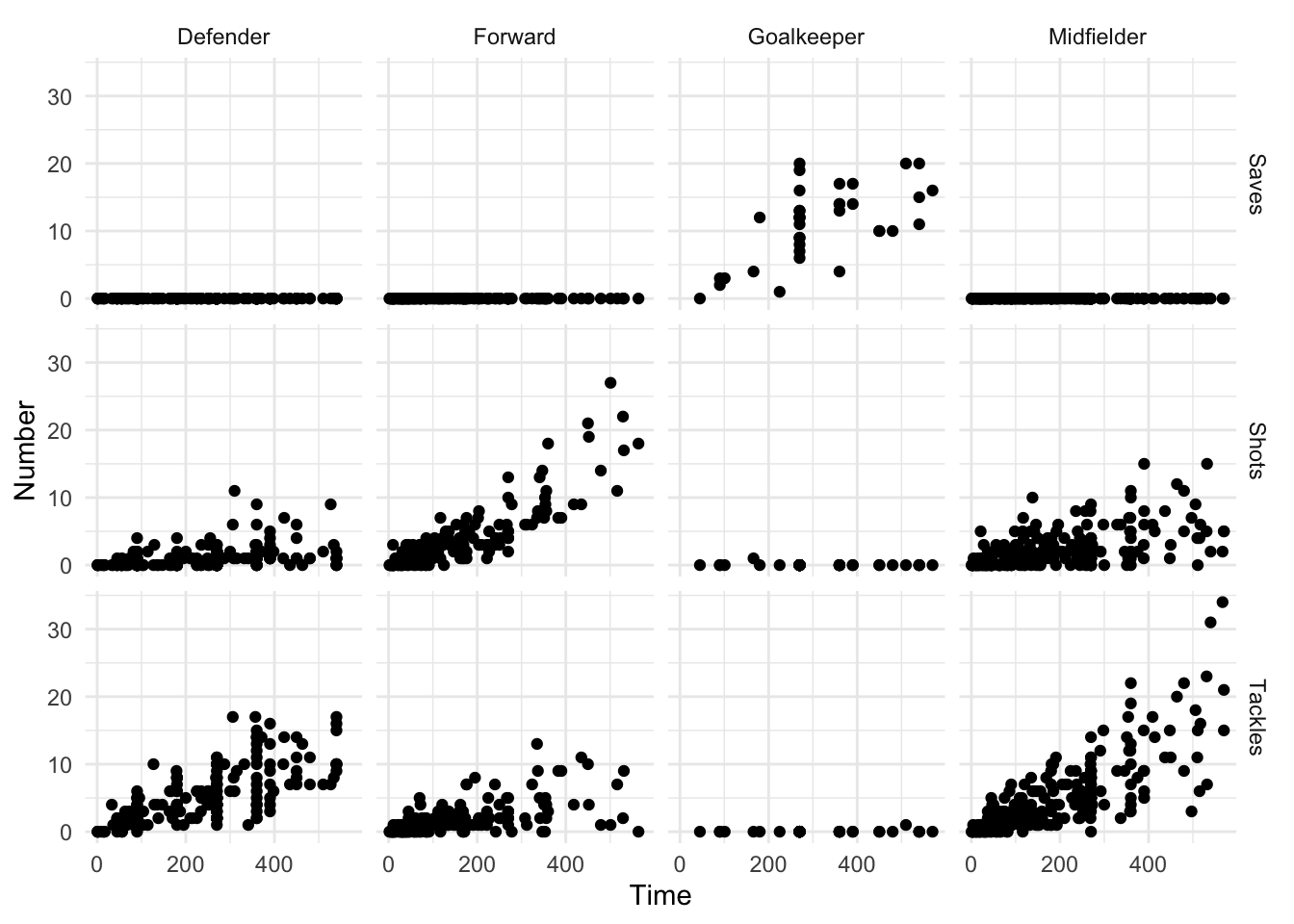
Figure 1.2: Example of a faceted plot created by taking advantage of the gather function to pull together data.
The spread function is less commonly needed to tidy data. It can, however, be useful for creating summary tables. For example, if you wanted to print a table of the average number and range of passes by position for the top four teams in this World Cup (Spain, Netherlands, Uruguay, and Germany), you could run:
library(knitr)

# Summarize the data to create the summary statistics you want
wc_table <- worldcup %>%
  filter(Team %in% c("Spain", "Netherlands", "Uruguay", "Germany")) %>%
  select(Team, Position, Passes) %>%
  group_by(Team, Position) %>%
  summarize(ave_passes = mean(Passes),
            min_passes = min(Passes),
            max_passes = max(Passes),
            pass_summary = paste0(round(ave_passes), " (",
                                  min_passes, ", ",
                                  max_passes, ")")) %>%
  select(Team, Position, pass_summary)
`summarise()` regrouping output by 'Team' (override with `.groups` argument)
# What the data looks like before using `spread`
wc_table
# A tibble: 16 x 3
# Groups:   Team [4]
   Team        Position   pass_summary
   <fct>       <fct>      <chr>
 1 Germany     Defender   190 (44, 360)
 2 Germany     Forward    90 (5, 217)
 3 Germany     Goalkeeper 99 (99, 99)
 4 Germany     Midfielder 177 (6, 423)
 5 Netherlands Defender   182 (30, 271)
 6 Netherlands Forward    97 (12, 248)
 7 Netherlands Goalkeeper 149 (149, 149)
 8 Netherlands Midfielder 170 (22, 307)
 9 Spain       Defender   213 (1, 402)
10 Spain       Forward    77 (12, 169)
11 Spain       Goalkeeper 67 (67, 67)
12 Spain       Midfielder 212 (16, 563)
13 Uruguay     Defender   83 (22, 141)
14 Uruguay     Forward    100 (5, 202)
15 Uruguay     Goalkeeper 75 (75, 75)
16 Uruguay     Midfielder 100 (1, 252)

# Use spread to create a prettier format for a table
wc_table %>%
  spread(Position, pass_summary) %>%
kable()| Team | Defender | Forward | Goalkeeper | Midfielder |
|---|---|---|---|---|
| Germany | 190 (44, 360) | 90 (5, 217) | 99 (99, 99) | 177 (6, 423) |
| Netherlands | 182 (30, 271) | 97 (12, 248) | 149 (149, 149) | 170 (22, 307) |
| Spain | 213 (1, 402) | 77 (12, 169) | 67 (67, 67) | 212 (16, 563) |
| Uruguay | 83 (22, 141) | 100 (5, 202) | 75 (75, 75) | 100 (1, 252) |
Notice in this example how spread has been used at the very end of the code sequence to convert the summarized data into a shape that offers a better tabular presentation for a report. In the spread call, you first specify the name of the column to use for the new column names (Position in this example) and then specify the column to use for the cell values (pass_summary here).
A> In this code, I’ve used the kable function from the knitr package to create the summary table in a table format, rather than as basic R output. This function is very useful for formatting basic tables in R markdown documents. For more complex tables, check out the pander and xtable packages.
1.5.6 Merging datasets
Often, you will have data in two separate datasets that you’d like to combine based on a common variable or variables. For example, for the World Cup example data we’ve been using, it would be interesting to add in a column with the final standing of each player’s team. We’ve included data with that information in a file called “team_standings.csv,” which can be read into the R object team_standings with the call:
team_standings <- read_csv("data/team_standings.csv")
team_standings %>% slice(1:3)
# A tibble: 3 x 2
  Standing Team
     <dbl> <chr>
1        1 Spain
2        2 Netherlands
3        3 Germany
This data frame has one observation per team, and the team names are consistent with the team names in the worldcup data frame.
You can use the different functions from the *_join family to merge this team standing data with the player statistics in the worldcup data frame. Once you’ve done that, you can use other data cleaning tools from dplyr to quickly pull and explore interesting parts of the dataset. The main arguments for the *_join functions are the object names of the two data frames to join and by, which specifies which variables to use to match up observations from the two dataframes.
There are several functions in the *_join family. These functions all merge together two data frames; they differ in how they handle observations that exist in one but not both data frames. Here are the four functions from this family that you will likely use the most often:
| Function | What it includes in merged data frame |
|---|---|
left_join |
Includes all observations in the left data frame, whether or not there is a match in the right data frame |
right_join |
Includes all observations in the right data frame, whether or not there is a match in the left data frame |
inner_join |
Includes only observations that are in both data frames |
full_join |
Includes all observations from both data frames |
In this table, the “left” data frame refers to the first data frame input in the *_join call, while the “right” data frame refers to the second data frame input into the function. For example, in the call
left_join(world_cup, team_standings, by = "Team")the world_cup data frame is the “left” data frame and the team_standings data frame is the “right” data frame. Therefore, using left_join would include all rows from world_cup, whether or not the player had a team listed in team_standings, while right_join would include all the rows from team_standings, whether or not there were any players from that team in world_cup.
W> Remember that if you are using piping, the first data frame (“left” for these functions) is by default the dataframe created by the code right before the pipe. When you merge data frames as a step in piped code, therefore, the “left” data frame is the one piped into the function while the “right” data frame is the one stated in the *_join function call.
As an example of merging, say you want to create a table of the top 5 players by shots on goal, as well as the final standing for each of these player’s teams, using the worldcup and team_standings data. You can do this by running:
data(worldcup)
worldcup %>%
  mutate(Name = rownames(worldcup),
         Team = as.character(Team)) %>%
  select(Name, Position, Shots, Team) %>%
  arrange(desc(Shots)) %>%
  slice(1:5) %>%
  left_join(team_standings, by = "Team") %>% # Merge in team standings
  rename("Team Standing" = Standing) %>%
kable()| Name | Position | Shots | Team | Team Standing |
|---|---|---|---|---|
| Gyan | Forward | 27 | Ghana | 7 |
| Villa | Forward | 22 | Spain | 1 |
| Messi | Forward | 21 | Argentina | 5 |
| Suarez | Forward | 19 | Uruguay | 4 |
| Forlan | Forward | 18 | Uruguay | 4 |
In addition to the merging in this code, there are a few other interesting things to point out:
- The code uses the
as.characterfunction within amutatecall to change the team name from a factor to a character in theworldcupdata frame. When merging two data frames, it’s safest if the column you’re using to merge has the same class in each data frame. The “Team” column is a character class in theteam_standingsdata frame but a factor class in theworldcupdata frame, so this call converts that column to a character class inworldcup. Theleft_joinfunction will still perform a merge if you don’t include this call, but it will throw a warning that it is coercing the column inworldcupto a character vector. It’s generally safer to do this yourself explictly. - It uses the
selectfunction both to remove columns we’re not interested in and also to put the columns we want to keep in the order we’d like for the final table. - It uses
arrangefollowed bysliceto pull out the top 5 players and order them by number of shots. - For one of the column names, we want to use “Team Standing” rather than the current column name of “Standing.” This code uses
renameat the very end to make this change right before creating the table. You can also use thecol.namesargument in thekablefunction to customize all the column names in the final table, but thisrenamecall is a quick fix since we just want to change one column name.