8 LECTURE: Tidy Data and the Tidyverse
The learning objectives for this section are to:
- Define tidy data and to transform non-tidy data into tidy data
One unifying concept of this book is the notion of tidy data. As defined by Hadley Wickham in his 2014 paper published in the Journal of Statistical Software, a tidy dataset has the following properties:
Each variable forms a column.
Each observation forms a row.
Each type of observational unit forms a table.
The purpose of defining tidy data is to highlight the fact that most data do not start out life as tidy. In fact, much of the work of data analysis may involve simply making the data tidy (at least this has been our experience). Once a dataset is tidy, it can be used as input into a variety of other functions that may transform, model, or visualize the data.
As a quick example, consider the following data illustrating death rates in Virginia in 1940 in a classic table format:
##       Rural Male Rural Female Urban Male Urban Female
## 50-54       11.7          8.7       15.4          8.4
## 55-59       18.1         11.7       24.3         13.6
## 60-64       26.9         20.3       37.0         19.3
## 65-69       41.0         30.9       54.6         35.1
## 70-74       66.0         54.3       71.1         50.0
While this format is canonical and is useful for quickly observing the relationship between multiple variables, it is not tidy. This format violates the tidy form because there are variables in both the rows and columns. In this case the variables are age category, gender, and urban-ness. Finally, the death rate itself, which is the fourth variable, is presented inside the table.
Converting this data to tidy format would give us
library(tidyverse)

VADeaths %>%
  as_tibble() %>%
  mutate(age = row.names(VADeaths)) %>%
  pivot_longer(-age) %>%
  separate(name, c("urban", "gender"), sep = " ") %>%
  mutate(age = factor(age), urban = factor(urban), gender = factor(gender))
## # A tibble: 20 x 4
## age urban gender value
## <fct> <fct> <fct> <dbl>
## 1 50-54 Rural Male 11.7
## 2 50-54 Rural Female 8.7
## 3 50-54 Urban Male 15.4
## 4 50-54 Urban Female 8.4
## 5 55-59 Rural Male 18.1
## 6 55-59 Rural Female 11.7
## 7 55-59 Urban Male 24.3
## 8 55-59 Urban Female 13.6
## 9 60-64 Rural Male 26.9
## 10 60-64 Rural Female 20.3
## 11 60-64 Urban Male 37
## 12 60-64 Urban Female 19.3
## 13 65-69 Rural Male 41
## 14 65-69 Rural Female 30.9
## 15 65-69 Urban Male 54.6
## 16 65-69 Urban Female 35.1
## 17 70-74 Rural Male 66
## 18 70-74 Rural Female 54.3
## 19 70-74 Urban Male 71.1
## 20 70-74 Urban Female 508.1 The “Tidyverse”
There are a number of R packages that take advantage of the tidy data form and can be used to do interesting things with data. Many (but not all) of these packages are written by Hadley Wickham and the collection of packages is sometimes referred to as the “tidyverse” because of their dependence on and presumption of tidy data. “Tidyverse” packages include
ggplot2: a plotting system based on the grammar of graphics
magrittr: defines the
%>%operator for chaining functions together in a series of operations on datadplyr: a suite of (fast) functions for working with data frames
tidyr: easily tidy data with
pivot_wider()andpivot_longer()functions
We will be using these packages extensively in this book.
The “tidyverse” package can be used to install all of the packages in the tidyverse at once. For example, instead of starting an R script with this:
You can start with this:
8.2 Reading Tabular Data with the readr Package
The learning objectives for this section are to:
- Read tabular data into R and read in web data via web scraping tools and APIs
The readr package is the primary means by which we will read tablular data, most notably, comma-separated-value (CSV) files. The readr package has a few functions in it for reading and writing tabular data—we will focus on the read_csv function. The readr package is available on CRAN and the code for the package is maintained on GitHub.
The importance of the read_csv function is perhaps better understood from an historical perspective. R’s built in read.csv function similarly reads CSV files, but the read_csv function in readr builds on that by removing some of the quirks and “gotchas” of read.csv as well as dramatically optimizing the speed with which it can read data into R. The read_csv function also adds some nice user-oriented features like a progress meter and a compact method for specifying column types.
The only required argument to read_csv is a character string specifying the path to the file to read. A typical call to read_csv will look as follows.
##
## ── Column specification ────────────────────────────────────────────────────────
## cols(
##   Standing = col_double(),
##   Team = col_character()
## )## # A tibble: 32 x 2
## Standing Team
## <dbl> <chr>
## 1 1 Spain
## 2 2 Netherlands
## 3 3 Germany
## 4 4 Uruguay
## 5 5 Argentina
## 6 6 Brazil
## 7 7 Ghana
## 8 8 Paraguay
## 9 9 Japan
## 10 10 Chile
## # … with 22 more rowsBy default, read_csv will open a CSV file and read it in line-by-line. It will also (by default), read in the first few rows of the table in order to figure out the type of each column (i.e. integer, character, etc.). In the code example above, you can see that read_csv has correctly assigned an integer class to the “Standing” variable in the input data and a character class to the “Team” variable. From the read_csv help page:
If [the argument for
col_typesis] ‘NULL’, all column types will be imputed from the first 1000 rows on the input. This is convenient (and fast), but not robust. If the imputation fails, you’ll need to supply the correct types yourself.
You can also specify the type of each column with the col_types argument. In general, it’s a good idea to specify the column types explicitly. This rules out any possible guessing errors on the part of read_csv. Also, specifying the column types explicitly provides a useful safety check in case anything about the dataset should change without you knowing about it.
Note that the col_types argument accepts a compact representation. Here "cc" indicates that the first column is character and the second column is character (there are only two columns). Using the col_types argument is useful because often it is not easy to automatically figure out the type of a column by looking at a few rows (especially if a column has many missing values).
The read_csv function will also read compressed files automatically. There is no need to decompress the file first or use the gzfile connection function. The following call reads a gzip-compressed CSV file containing download logs from the RStudio CRAN mirror.
##
## ── Column specification ────────────────────────────────────────────────────────
## cols(
##   date = col_date(format = ""),
##   time = col_time(format = ""),
##   size = col_double(),
##   r_version = col_character(),
##   r_arch = col_character(),
##   r_os = col_character(),
##   package = col_character(),
##   version = col_character(),
##   country = col_character(),
##   ip_id = col_double()
## )
Note that the message (“Parse with column specification …”) printed after the call indicates that read_csv may have had some difficulty identifying the type of each column. This can be solved by using the col_types argument.
## # A tibble: 10 x 10
##    date    time      size r_version r_arch r_os   package  version country ip_id
##    <chr>   <chr>    <int> <chr>     <chr>  <chr>  <chr>    <chr>   <chr>   <int>
##  1 2016-0… 06:04…  144723 3.3.1     i386   mingw… gtools   3.5.0   US          1
##  2 2016-0… 06:04… 2049711 3.3.0     i386   mingw… rmarkdo… 1.0     DK          2
##  3 2016-0… 06:04…   26252 <NA>      <NA>   <NA>   R.metho… 1.7.1   AU          3
##  4 2016-0… 06:04…  556091 2.13.1    x86_64 mingw… tibble   1.1     CN          4
##  5 2016-0… 06:03…  313363 2.13.1    x86_64 mingw… iterato… 1.0.5   US          5
##  6 2016-0… 06:03…  378892 3.3.1     x86_64 mingw… foreach  1.3.2   US          5
##  7 2016-0… 06:04…   41228 3.3.1     x86_64 linux… moments  0.14    US          6
##  8 2016-0… 06:04…  403177 <NA>      <NA>   <NA>   R.oo     1.20.0  AU          3
##  9 2016-0… 06:04…     525 3.3.0     x86_64 linux… rgl      0.95.1… KR          7
## 10 2016-0… 06:04…  755720 3.2.5     x86_64 mingw… geosphe… 1.5-5   US          8
You can specify the column type in a more detailed fashion by using the various col_* functions. For example, in the log data above, the first column is actually a date, so it might make more sense to read it in as a Date variable. If we wanted to just read in that first column, we could do
logdates <- read_csv("data/2016-07-20.csv.gz",
                     col_types = cols_only(date = col_date()),
                     n_max = 10)
logdates
## # A tibble: 10 x 1
## date
## <date>
## 1 2016-07-20
## 2 2016-07-20
## 3 2016-07-20
## 4 2016-07-20
## 5 2016-07-20
## 6 2016-07-20
## 7 2016-07-20
## 8 2016-07-20
## 9 2016-07-20
## 10 2016-07-20Now the date column is stored as a Date object which can be used for relevant date-related computations (for example, see the lubridate package).
The read_csv function has a progress option that defaults to TRUE. This options provides a nice progress meter while the CSV file is being read. However, if you are using read_csv in a function, or perhaps embedding it in a loop, it’s probably best to set progress = FALSE.
The readr package includes a variety of functions in the read_* family that allow you to read in data from different formats of flat files. The following table gives a guide to several functions in the read_* family.
readr function |
Use |
|---|---|
read_csv |
Reads comma-separated file |
read_csv2 |
Reads semicolon-separated file |
read_tsv |
Reads tab-separated file |
read_delim |
General function for reading delimited files |
read_fwf |
Reads fixed width files |
read_log |
Reads log files |
8.3 Reading Web-Based Data
The learning objectives for this section are to:
- Read in web data via web scraping tools and APIs
Not only can you read in data locally stored on your computer, with R it is also fairly easy to read in data stored on the web.
8.3.1 Flat files online
The simplest way to do this is if the data is available online as a flat file (see note below). For example, the “Extended Best Tracks” for the North Atlantic are hurricane tracks that include both the best estimate of the central location of each storm and also gives estimates of how far winds of certain speeds extended from the storm’s center in four quadrants of the storm (northeast, northwest, southeast, southwest) at each measurement point. You can see this file online here.
How can you tell if you’ve found a flat file online? Here are a couple of clues:
- It will not have any formatting. Instead, it will look online as if you opened a file in a text editor on your own computer.
-
It will often have a web address that ends with a typical flat file extension (
“.csv”,“.txt”, or“.fwf”, for example).
Here are a couple of examples of flat files available online:
If you copy and paste the web address for this file, you’ll see that the url for this example hurricane data file is non-secure (starts with http:) and that it ends with a typical flat file extension (.txt, in this case). You can read this file into your R session using the same readr function that you would use to read it in if the file were stored on your computer.
First, you can create an R object with the filepath to the file. In the case of online files, that’s the url. To fit the long web address comfortably in an R script window, you can use the paste0 function to paste pieces of the web address together:
ext_tracks_file <- paste0("http://rammb.cira.colostate.edu/research/",
                          "tropical_cyclones/tc_extended_best_track_dataset/",
                          "data/ebtrk_atlc_1988_2015.txt")
Next, since this web-based file is a fixed width file, you’ll need to define the width of each column, so that R will know where to split between columns. You can then use the read_fwf function from the readr package to read the file into your R session. This data, like a lot of weather data, uses the string "-99" for missing data, and you can specify that missing value character with the na argument in read_fwf. Also, the online file does not include column names, so you’ll have to use the data documentation file for the dataset to determine and set those yourself.
library(readr)

# Create a vector of the width of each column
ext_tracks_widths <- c(7, 10, 2, 2, 3, 5, 5, 6, 4, 5, 4, 4, 5, 3, 4, 3, 3, 3,
                       4, 3, 3, 3, 4, 3, 3, 3, 2, 6, 1)

# Create a vector of column names, based on the online documentation for this data
ext_tracks_colnames <- c("storm_id", "storm_name", "month", "day",
                          "hour", "year", "latitude", "longitude",
                          "max_wind", "min_pressure", "rad_max_wind",
                          "eye_diameter", "pressure_1", "pressure_2",
                          paste("radius_34", c("ne", "se", "sw", "nw"), sep = "_"),
                          paste("radius_50", c("ne", "se", "sw", "nw"), sep = "_"),
                          paste("radius_64", c("ne", "se", "sw", "nw"), sep = "_"),
                          "storm_type", "distance_to_land", "final")

# Read the file in from its url
ext_tracks <- read_fwf(ext_tracks_file,
                       fwf_widths(ext_tracks_widths, ext_tracks_colnames),
                       na = "-99")
ext_tracks[1:3, 1:9]
## # A tibble: 3 x 9
## storm_id storm_name month day hour year latitude longitude max_wind
## <chr> <chr> <chr> <chr> <chr> <dbl> <dbl> <dbl> <dbl>
## 1 AL0188 ALBERTO 08 05 18 1988 32 77.5 20
## 2 AL0188 ALBERTO 08 06 00 1988 32.8 76.2 20
## 3 AL0188 ALBERTO 08 06 06 1988 34 75.2 20
For some fixed width files, you may be able to save the trouble of counting column widths by using the fwf_empty function in the readr package. This function guesses the widths of columns based on the positions of empty columns. However, the example hurricane dataset we are using here is a bit too messy for this– in some cases, there are values from different columns that are not separated by white space. Just as it is typically safer for you to specify column types yourself, rather than relying on R to correctly guess them, it is also safer when reading in a fixed width file to specify column widths yourself.
You can use some dplyr functions to check out the dataset once it’s in R (there will be much more about dplyr in the next section). For example, the following call prints a sample of four rows of data from Hurricane Katrina, with, for each row, the date and time, maximum wind speed, minimum pressure, and the radius of maximum winds of the storm for that observation:
library(dplyr)

ext_tracks %>%
  filter(storm_name == "KATRINA") %>%
  select(month, day, hour, max_wind, min_pressure, rad_max_wind) %>%
  sample_n(4)
## # A tibble: 4 x 6
## month day hour max_wind min_pressure rad_max_wind
## <chr> <chr> <chr> <dbl> <dbl> <dbl>
## 1 11 01 06 20 1011 90
## 2 10 29 00 30 1001 40
## 3 08 30 12 30 985 30
## 4 08 31 06 25 996 NAWith the functions in the readr package, you can also read in flat files from secure urls (ones that starts with https:). (This is not true with the read.table family of functions from base R.) One example where it is common to find flat files on secure sites is on GitHub. If you find a file with a flat file extension in a GitHub repository, you can usually click on it and then choose to view the “Raw” version of the file, and get to the flat file version of the file.
For example, the CDC Epidemic Prediction Initiative has a GitHub repository with data on Zika cases, including files on cases in Brazil. When we wrote this, the most current file was available here, with the raw version (i.e., a flat file) available by clicking the “Raw” button on the top right of the first site.
zika_file <- paste0("https://raw.githubusercontent.com/cdcepi/zika/master/",
                    "Brazil/COES_Microcephaly/data/COES_Microcephaly-2016-06-25.csv")
zika_brazil <- read_csv(zika_file)

zika_brazil %>%
  select(location, value, unit)
## # A tibble: 210 x 3
## location value unit
## <chr> <dbl> <chr>
## 1 Brazil-Acre 2 cases
## 2 Brazil-Alagoas 75 cases
## 3 Brazil-Amapa 7 cases
## 4 Brazil-Amazonas 8 cases
## 5 Brazil-Bahia 263 cases
## 6 Brazil-Ceara 124 cases
## 7 Brazil-Distrito_Federal 5 cases
## 8 Brazil-Espirito_Santo 13 cases
## 9 Brazil-Goias 14 cases
## 10 Brazil-Maranhao 131 cases
## # … with 200 more rows8.3.2 Requesting data through a web API
Web APIs are growing in popularity as a way to access open data from government agencies, companies, and other organizations. “API” stands for “Application Program Interface”"; an API provides the rules for software applications to interact. In the case of open data APIs, they provide the rules you need to know to write R code to request and pull data from the organization’s web server into your R session. Usually, some of the computational burden of querying and subsetting the data is taken on by the source’s server, to create the subset of requested data to pass to your computer. In practice, this means you can often pull the subset of data you want from a very large available dataset without having to download the full dataset and load it locally into your R session.
As an overview, the basic steps for accessing and using data from a web API when working in R are:
- Figure out the API rules for HTTP requests
- Write R code to create a request in the proper format
- Send the request using GET or POST HTTP methods
- Once you get back data from the request, parse it into an easier-to-use format if necessary
To get the data from an API, you should first read the organization’s API documentation. An organization will post details on what data is available through their API(s), as well as how to set up HTTP requests to get that data– to request the data through the API, you will typically need to send the organization’s web server an HTTP request using a GET or POST method. The API documentation details will typically show an example GET or POST request for the API, including the base URL to use and the possible query parameters that can be used to customize the dataset request.
For example, the National Aeronautics and Space Administration (NASA) has an API for pulling the Astronomy Picture of the Day. In their API documentation, they specify that the base URL for the API request should be “https://api.nasa.gov/planetary/apod” and that you can include parameters to specify the date of the daily picture you want, whether to pull a high-resolution version of the picture, and a NOAA API key you have requested from NOAA.
Many organizations will require you to get an API key and use this key in each of your API requests. This key allows the organization to control API access, including enforcing rate limits per user. API rate limits restrict how often you can request data (e.g., an hourly limit of 1,000 requests per user for NASA APIs).
API keys should be kept private, so if you are writing code that includes an API key, be very careful not to include the actual key in any code made public (including any code in public GitHub repositories). One way to do this is to save the value of your key in a file named .Renviron in your home directory. This file should be a plain text file and must end in a blank line. Once you’ve saved your API key to a global variable in that file (e.g., with a line added to the .Renviron file like NOAA_API_KEY="abdafjsiopnab038"), you can assign the key value to an R object in an R session using the Sys.getenv function (e.g., noaa_api_key <- Sys.getenv("NOAA_API_KEY")), and then use this object (noaa_api_key) anywhere you would otherwise have used the character string with your API key.
To find more R packages for accessing and exploring open data, check out the Open Data CRAN task view. You can also browse through the ROpenSci packages, all of which have GitHub repositories where you can further explore how each package works. ROpenSci is an organization with the mission to create open software tools for science. If you create your own package to access data relevant to scientific research through an API, consider submitting it for peer-review through ROpenSci.
The riem package, developed by Maelle Salmon and an ROpenSci package, is an excellent and straightforward example of how you can use R to pull open data through a web API. This package allows you to pull weather data from airports around the world directly from the Iowa Environmental Mesonet. To show you how to pull data into R through an API, in this section we will walk you through code in the riem package or code based closely on code in the package.
To get a certain set of weather data from the Iowa Environmental Mesonet, you can send an HTTP request specifying a base URL, “https://mesonet.agron.iastate.edu/cgi-bin/request/asos.py/”, as well as some parameters describing the subset of dataset you want (e.g., date ranges, weather variables, output format). Once you know the rules for the names and possible values of these parameters (more on that below), you can submit an HTTP GET request using the GET function from the httr package.
When you are making an HTTP request using the GET or POST functions from the httr package, you can include the key-value pairs for any query parameters as a list object in the query argurment of the function. For example, suppose you want to get wind speed in miles per hour (data = "sped") for Denver, CO, (station = "DEN") for the month of June 2016 (year1 = "2016", month1 = "6", etc.) in Denver’s local time zone (tz = "America/Denver") and in a comma-separated file (format = "comma"). To get this weather dataset, you can run:
library(httr)
meso_url <- "https://mesonet.agron.iastate.edu/cgi-bin/request/asos.py/"
denver <- GET(url = meso_url,
                    query = list(station = "DEN",
                                 data = "sped",
                                 year1 = "2016",
                                 month1 = "6",
                                 day1 = "1",
                                 year2 = "2016",
                                 month2 = "6",
                                 day2 = "30",
                                 tz = "America/Denver",
                                 format = "comma")) %>%
  content() %>%
  read_csv(skip = 5, na = "M")

denver %>% slice(1:3)
## # A tibble: 3 x 3
## station valid sped
## <chr> <dttm> <dbl>
## 1 DEN 2016-06-01 00:00:00 9.2
## 2 DEN 2016-06-01 00:05:00 9.2
## 3 DEN 2016-06-01 00:10:00 6.9
The content call in this code extracts the content from the response to the HTTP request sent by the GET function. The Iowa Environmental Mesonet API offers the option to return the requested data in a comma-separated file (format = “comma” in the GET request), so here content and read_csv are used to extract and read in that csv file. Usually, data will be returned in a JSON format instead. We include more details later in this section on parsing data returned in a JSON format.
The only tricky part of this process is figuring out the available parameter names (e.g., station) and possible values for each (e.g., "DEN" for Denver). Currently, the details you can send in an HTTP request through Iowa Environmental Mesonet’s API include:
- A four-character weather station identifier (
station) - The weather variables (e.g., temperature, wind speed) to include (
data) - Starting and ending dates describing the range for which you’d like to pull data (
year1,month1,day1,year2,month2,day2) - The time zone to use for date-times for the weather observations (
tz) - Different formatting options (e.g., delimiter to use in the resulting data file [
format], whether to include longitude and latitude)
Typically, these parameter names and possible values are explained in the API documentation. In some cases, however, the documentation will be limited. In that case, you may be able to figure out possible values, especially if the API specifies a GET rather than POST method, by playing around with the website’s point-and-click interface and then looking at the url for the resulting data pages. For example, if you look at the Iowa Environmental Mesonet’s page for accessing this data, you’ll notice that the point-and-click web interface allows you the options in the list above, and if you click through to access a dataset using this interface, the web address of the data page includes these parameter names and values.
The riem package implements all these ideas in three very clean and straightforward functions. You can explore the code behind this package and see how these ideas can be incorporated into a small R package, in the /R directory of the package’s GitHub page.
R packages already exist for many open data APIs. If an R package already exists for an API, you can use functions from that package directly, rather than writing your own code using the API protocols and httr functions. Other examples of existing R packages to interact with open data APIs include:
twitteR: Twitterrnoaa: National Oceanic and Atmospheric AdministrationQuandl: Quandl (financial data)RGoogleAnalytics: Google Analyticscensusr,acs: United States CensusWDI,wbstats: World BankGuardianR,rdian: The Guardian Media GroupblsAPI: Bureau of Labor Statisticsrtimes: New York TimesdataRetrieval,waterData: United States Geological Survey
If an R package doesn’t exist for an open API and you’d like to write your own package, find out more about writing API packages with this vignette for the httr package. This document includes advice on error handling within R code that accesses data through an open API.
8.3.3 Scraping web data
You can also use R to pull and clean web-based data that is not accessible through a web API or as an online flat file. In this case, the strategy will often be to pull in the full web page file (often in HTML or XML) and then parse or clean it within R.
The rvest package is a good entry point for handling more complex collection and cleaning of web-based data. This package includes functions, for example, that allow you to select certain elements from the code for a web page (e.g., using the html_node and xml_node functions), to parse tables in an HTML document into R data frames (html_table), and to parse, fill out, and submit HTML forms (html_form, set_values, submit_form). Further details on web scraping with R are beyond the scope of this course, but if you’re interested, you can find out more through the rvest GitHub README.
8.3.4 Parsing JSON, XML, or HTML data
Often, data collected from the web, including the data returned from an open API or obtained by scraping a web page, will be in JSON, XML, or HTML format. To use data in a JSON, XML, or HTML format in R, you need to parse the file from its current format and convert it into an R object more useful for analysis.
Typically, JSON-, XML-, or HTML-formatted data is parsed into a list in R, since list objects allow for a lot of flexibility in the structure of the data. However, if the data is structured appropriately, you can often parse data into another type of object (a data frame, for example, if the data fits well into a two-dimensional format of rows and columns). If the data structure of the data that you are pulling in is complex but consistent across different observations, you may alternatively want to create a custom object type to parse the data into.
There are a number of packages for parsing data from these formats, including jsonlite and xml2. To find out more about parsing data from typical web formats, and for more on working with web-based documents and data, see the CRAN task view for Web Technologies and Services
8.4 Basic Data Manipulation
The learning objectives for this section are to:
- Transform non-tidy data into tidy data
- Manipulate and transform a variety of data types, including dates, times, and text data
The two packages dplyr and tidyr, both “tidyverse” packages, allow you to quickly and fairly easily clean up your data. These packages are not very old, and so much of the example R code you might find in books or online might not use the functions we use in examples in this section (although this is quickly changing for new books and for online examples). Further, there are many people who are used to using R base functionality to clean up their data, and some of them still do not use these packages much when cleaning data. We think, however, that dplyr is easier for people new to R to learn than learning how to clean up data using base R functions, and we also think it produces code that is much easier to read, which is useful in maintaining and sharing code.
For many of the examples in this section, we will use the ext_tracks hurricane dataset we input from a url as an example in a previous section of this book. If you need to load a version of that data, we have also saved it locally, so you can create an R object with the example data for this section by running:
ext_tracks_file <- "data/ebtrk_atlc_1988_2015.txt"
ext_tracks_widths <- c(7, 10, 2, 2, 3, 5, 5, 6, 4, 5, 4, 4, 5, 3, 4, 3, 3, 3,
                       4, 3, 3, 3, 4, 3, 3, 3, 2, 6, 1)
ext_tracks_colnames <- c("storm_id", "storm_name", "month", "day",
                          "hour", "year", "latitude", "longitude",
                          "max_wind", "min_pressure", "rad_max_wind",
                          "eye_diameter", "pressure_1", "pressure_2",
                          paste("radius_34", c("ne", "se", "sw", "nw"), sep = "_"),
                          paste("radius_50", c("ne", "se", "sw", "nw"), sep = "_"),
                          paste("radius_64", c("ne", "se", "sw", "nw"), sep = "_"),
                          "storm_type", "distance_to_land", "final")
ext_tracks <- read_fwf(ext_tracks_file,
                       fwf_widths(ext_tracks_widths, ext_tracks_colnames),
                       na = "-99")
8.4.1 Piping
The dplyr and tidyr functions are often used in conjunction with piping, which is done with the %>% function from the magrittr package. Piping can be done with many R functions, but is especially common with dplyr and tidyr functions. The concept is straightforward– the pipe passes the data frame output that results from the function right before the pipe to input it as the first argument of the function right after the pipe.
Here is a generic view of how this works in code, for a pseudo-function named function that inputs a data frame as its first argument:
# Without piping
function(dataframe, argument_2, argument_3)

# With piping
dataframe %>%
  function(argument_2, argument_3)
For example, without piping, if you wanted to see the time, date, and maximum winds for Katrina from the first three rows of the ext_tracks hurricane data, you could run:
katrina <- filter(ext_tracks, storm_name == "KATRINA")
katrina_reduced <- select(katrina, month, day, hour, max_wind)
head(katrina_reduced, 3)
## # A tibble: 3 x 4
## month day hour max_wind
## <chr> <chr> <chr> <dbl>
## 1 10 28 18 30
## 2 10 29 00 30
## 3 10 29 06 30In this code, you are creating new R objects at each step, which makes the code cluttered and also requires copying the data frame several times into memory. As an alternative, you could just wrap one function inside another:
## # A tibble: 3 x 4
##   month day   hour  max_wind
##   <chr> <chr> <chr>    <dbl>
## 1 10    28    18          30
## 2 10    29    00          30
## 3 10 29 06 30This avoids re-assigning the data frame at each step, but quickly becomes ungainly, and it’s easy to put arguments in the wrong layer of parentheses. Piping avoids these problems, since at each step you can send the output from the last function into the next function as that next function’s first argument:
## # A tibble: 3 x 4
##   month day   hour  max_wind
##   <chr> <chr> <chr>    <dbl>
## 1 10    28    18          30
## 2 10    29    00          30
## 3 10 29 06 308.4.2 Summarizing data
The dplyr and tidyr packages have numerous functions (sometimes referred to as “verbs”) for cleaning up data. We’ll start with the functions to summarize data.
The primary of these is summarize, which inputs a data frame and creates a new data frame with the requested summaries. In conjunction with summarize, you can use other functions from dplyr (e.g., n, which counts the number of observations in a given column) to create this summary. You can also use R functions from other packages or base R functions to create the summary.
For example, say we want a summary of the number of observations in the ext_tracks hurricane dataset, as well as the highest measured maximum windspeed (given by the column max_wind in the dataset) in any of the storms, and the lowest minimum pressure (min_pressure). To create this summary, you can run:
ext_tracks %>%
  summarize(n_obs = n(),
            worst_wind = max(max_wind),
            worst_pressure = min(min_pressure))
## # A tibble: 1 x 3
## n_obs worst_wind worst_pressure
## <int> <dbl> <dbl>
## 1 11824 160 0This summary provides particularly useful information for this example data, because it gives an unrealistic value for minimum pressure (0 hPa). This shows that this dataset will need some cleaning. The highest wind speed observed for any of the storms, 160 knots, is more reasonable.
You can also use summarize with functions you’ve written yourself, which gives you a lot of power in summarizing data in interesting ways. As a simple example, if you wanted to present the maximum wind speed in the summary above using miles per hour rather than knots, you could write a function to perform the conversion, and then use that function within the summarize call:
knots_to_mph <- function(knots){
  mph <- 1.152 * knots
}

ext_tracks %>%
  summarize(n_obs = n(),
            worst_wind = knots_to_mph(max(max_wind)),
            worst_pressure = min(min_pressure))
## # A tibble: 1 x 3
## n_obs worst_wind worst_pressure
## <int> <dbl> <dbl>
## 1 11824 184. 0So far, we’ve only used summarize to create a single-line summary of the data frame. In other words, the summary functions are applied across the entire dataset, to return a single value for each summary statistic. However, often you might want summaries stratified by a certain grouping characteristic of the data. For the hurricane data, for example, you might want to get the worst wind and worst pressure by storm, rather than across all storms.
You can do this by grouping your data frame by one of its column variables, using the function group_by, and then using summarize. The group_by function does not make a visible change to a data frame, although you can see, if you print out a grouped data frame, that the new grouping variable will be listed under “Groups” at the top of a print-out:
## # A tibble: 6 x 29
## # Groups:   storm_name, year [1]
##   storm_id storm_name month day   hour   year latitude longitude max_wind
##   <chr>    <chr>      <chr> <chr> <chr> <dbl>    <dbl>     <dbl>    <dbl>
## 1 AL0188   ALBERTO    08    05    18     1988     32        77.5       20
## 2 AL0188   ALBERTO    08    06    00     1988     32.8      76.2       20
## 3 AL0188   ALBERTO    08    06    06     1988     34        75.2       20
## 4 AL0188   ALBERTO    08    06    12     1988     35.2      74.6       25
## 5 AL0188   ALBERTO    08    06    18     1988     37        73.5       25
## 6 AL0188   ALBERTO    08    07    00     1988     38.7      72.4       25
## # … with 20 more variables: min_pressure <dbl>, rad_max_wind <dbl>,
## #   eye_diameter <dbl>, pressure_1 <dbl>, pressure_2 <dbl>, radius_34_ne <dbl>,
## #   radius_34_se <dbl>, radius_34_sw <dbl>, radius_34_nw <dbl>,
## #   radius_50_ne <dbl>, radius_50_se <dbl>, radius_50_sw <dbl>,
## #   radius_50_nw <dbl>, radius_64_ne <dbl>, radius_64_se <dbl>,
## #   radius_64_sw <dbl>, radius_64_nw <dbl>, storm_type <chr>,
## #   distance_to_land <dbl>, final <chr>
As a note, since hurricane storm names repeat at regular intervals until they are retired, to get a separate summary for each unique storm, this example requires grouping by both storm_name and year.
Even though applying the group_by function does not cause a noticeable change to the data frame itself, you’ll notice the difference in grouped and ungrouped data frames when you use summarize on the data frame. If a data frame is grouped, all summaries are calculated and given separately for each unique value of the grouping variable:
ext_tracks %>%
  group_by(storm_name, year) %>%
  summarize(n_obs = n(),
            worst_wind = max(max_wind),
            worst_pressure = min(min_pressure))
## `summarise()` regrouping output by 'storm_name' (override with `.groups` argument)## # A tibble: 378 x 5
## # Groups: storm_name [160]
## storm_name year n_obs worst_wind worst_pressure
## <chr> <dbl> <int> <dbl> <dbl>
## 1 ALBERTO 1988 13 35 1002
## 2 ALBERTO 1994 31 55 993
## 3 ALBERTO 2000 87 110 950
## 4 ALBERTO 2006 37 60 969
## 5 ALBERTO 2012 20 50 995
## 6 ALEX 1998 26 45 1002
## 7 ALEX 2004 25 105 957
## 8 ALEX 2010 30 90 948
## 9 ALLISON 1989 28 45 999
## 10 ALLISON 1995 33 65 982
## # … with 368 more rowsThis grouping / summarizing combination can be very useful for quickly plotting interesting summaries of a dataset. For example, to plot a histogram of maximum wind speed observed for each storm (Figure 8.1), you could run:
library(ggplot2)
ext_tracks %>%
  group_by(storm_name) %>%
  summarize(worst_wind = max(max_wind)) %>%
ggplot(aes(x = worst_wind)) + geom_histogram() 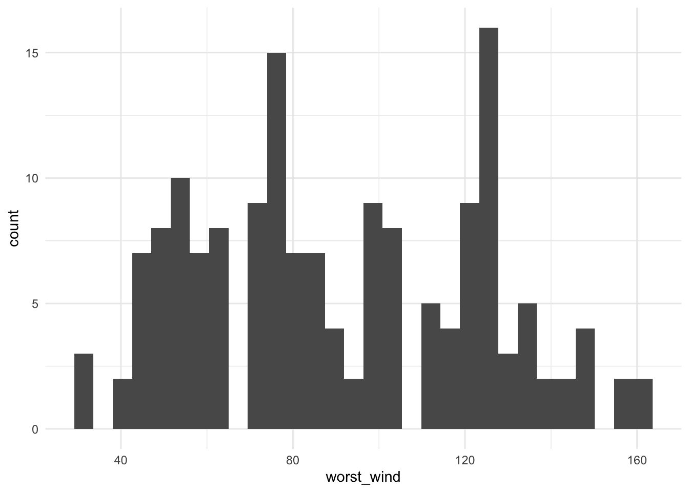
Figure 8.1: Histogram of the maximum wind speed observed during a storm for all Atlantic basin tropical storms, 1988–2015.
We will show a few basic examples of plotting using ggplot2 functions in this chapter of the book. We will cover plotting much more thoroughly in a later section.
From Figure 8.1, we can see that only two storms had maximum wind speeds at or above 160 knots (we’ll check this later with some other dplyr functions).
You cannot make changes to a variable that is being used to group a dataframe. If you try, you will get the error Error: cannot modify grouping variable. If you get this error, use the ungroup function to remove grouping within a data frame, and then you will be able to mutate any of the variables in the data.
8.4.3 Selecting and filtering data
When cleaning up data, you will need to be able to create subsets of the data, by selecting certain columns or filtering down to certain rows. These actions can be done using the dplyr functions select and filter.
The select function subsets certain columns of a data frame. The most basic way to use select is select certain columns by specifying their full column names. For example, to select the storm name, date, time, latitude, longitude, and maximum wind speed from the ext_tracks dataset, you can run:
## # A tibble: 11,824 x 8
##    storm_name month day   hour   year latitude longitude max_wind
##    <chr>      <chr> <chr> <chr> <dbl>    <dbl>     <dbl>    <dbl>
##  1 ALBERTO    08    05    18     1988     32        77.5       20
##  2 ALBERTO    08    06    00     1988     32.8      76.2       20
##  3 ALBERTO    08    06    06     1988     34        75.2       20
##  4 ALBERTO    08    06    12     1988     35.2      74.6       25
##  5 ALBERTO    08    06    18     1988     37        73.5       25
##  6 ALBERTO    08    07    00     1988     38.7      72.4       25
##  7 ALBERTO    08    07    06     1988     40        70.8       30
##  8 ALBERTO    08    07    12     1988     41.5      69         35
##  9 ALBERTO    08    07    18     1988     43        67.5       35
## 10 ALBERTO    08    08    00     1988     45        65.5       35
## # … with 11,814 more rows
There are several functions you can use with select that give you more flexibility, and so allow you to select columns without specifying the full names of each column. For example, the starts_with function can be used within a select function to pick out all the columns that start with a certain text string. As an example of using starts_with in conjunction with select, in the ext_tracks hurricane data, there are a number of columns that say how far from the storm center winds of certain speeds extend. Tropical storms often have asymmetrical wind fields, so these wind radii are given for each quadrant of the storm (northeast, southeast, northwest, and southeast of the storm’s center). All of the columns with the radius to which winds of 34 knots or more extend start with “radius_34”. To get a dataset with storm names, location, and radii of winds of 34 knots, you could run:
## # A tibble: 11,824 x 7
##    storm_name latitude longitude radius_34_ne radius_34_se radius_34_sw
##    <chr>         <dbl>     <dbl>        <dbl>        <dbl>        <dbl>
##  1 ALBERTO        32        77.5            0            0            0
##  2 ALBERTO        32.8      76.2            0            0            0
##  3 ALBERTO        34        75.2            0            0            0
##  4 ALBERTO        35.2      74.6            0            0            0
##  5 ALBERTO        37        73.5            0            0            0
##  6 ALBERTO        38.7      72.4            0            0            0
##  7 ALBERTO        40        70.8            0            0            0
##  8 ALBERTO        41.5      69            100          100           50
##  9 ALBERTO        43        67.5          100          100           50
## 10 ALBERTO        45        65.5           NA           NA           NA
## # … with 11,814 more rows, and 1 more variable: radius_34_nw <dbl>
Other functions that can be used with select in a similar way include:
ends_with: Select all columns that end with a certain string (for example,select(ext_tracks, ends_with("ne"))to get all the wind radii for the northeast quadrant of a storm for the hurricane example data)contains: Select all columns that include a certain string (select(ext_tracks, contains("34"))to get all wind radii for 34-knot winds)matches: Select all columns that match a certain relative expression (select(ext_tracks, matches("_[0-9][0-9]_"))to get all columns where the column name includes two numbers between two underscores, a pattern that matches all of the wind radii columns)
While select picks out certain columns of the data frame, filter picks out certain rows. With filter, you can specify certain conditions using R’s logical operators, and the function will return rows that meet those conditions.
R’s logical operators include:
| Operator | Meaning | Example |
|---|---|---|
== |
Equals | storm_name == KATRINA |
!= |
Does not equal | min_pressure != 0 |
> |
Greater than | latitude > 25 |
>= |
Greater than or equal to | max_wind >= 160 |
< |
Less than | min_pressure < 900 |
<= |
Less than or equal to | distance_to_land <= 0 |
%in% |
Included in | storm_name %in% c("KATRINA", "ANDREW") |
is.na() |
Is a missing value | is.na(radius_34_ne) |
If you are ever unsure of how to write a logical statement, but know how to write its opposite, you can use the ! operator to negate the whole statement. For example, if you wanted to get all storms except those named “KATRINA” and “ANDREW”, you could use !(storm_name %in% c("KATRINA", "ANDREW")). A common use of this is to identify observations with non-missing data (e.g., !(is.na(radius_34_ne))).
A logical statement, run by itself on a vector, will return a vector of the same length with TRUE every time the condition is met and FALSE every time it is not.
## [1] "18" "00" "06" "12" "18" "00"## [1] FALSE TRUE FALSE FALSE FALSE TRUEWhen you use a logical statement within filter, it will return just the rows where the logical statement is true:
## # A tibble: 9 x 3
##   storm_name hour  max_wind
##   <chr>      <chr>    <dbl>
## 1 ALBERTO    18          20
## 2 ALBERTO    00          20
## 3 ALBERTO    06          20
## 4 ALBERTO    12          25
## 5 ALBERTO    18          25
## 6 ALBERTO    00          25
## 7 ALBERTO    06          30
## 8 ALBERTO    12          35
## 9 ALBERTO 18 35## # A tibble: 3 x 3
## storm_name hour max_wind
## <chr> <chr> <dbl>
## 1 ALBERTO 00 20
## 2 ALBERTO 00 25
## 3 ALBERTO 00 35Filtering can also be done after summarizing data. For example, to determine which storms had maximum wind speed equal to or above 160 knots, run:
ext_tracks %>%
  group_by(storm_name, year) %>%
  summarize(worst_wind = max(max_wind)) %>%
  filter(worst_wind >= 160)
## `summarise()` regrouping output by 'storm_name' (override with `.groups` argument)## # A tibble: 2 x 3
## # Groups: storm_name [2]
## storm_name year worst_wind
## <chr> <dbl> <dbl>
## 1 GILBERT 1988 160
## 2 WILMA 2005 160If you would like to string several logical conditions together and select rows where all or any of the conditions are true, you can use the “and” (&) or “or” (|) operators. For example, to pull out observations for Hurricane Andrew when it was at or above Category 5 strength (137 knots or higher), you could run:
ext_tracks %>%
  select(storm_name, month, day, hour, latitude, longitude, max_wind) %>%
  filter(storm_name == "ANDREW" & max_wind >= 137)
## # A tibble: 2 x 7
## storm_name month day hour latitude longitude max_wind
## <chr> <chr> <chr> <chr> <dbl> <dbl> <dbl>
## 1 ANDREW 08 23 12 25.4 74.2 145
## 2 ANDREW 08 23 18 25.4 75.8 150Some common errors that come up when using logical operators in R are:
-
If you want to check that two things are equal, make sure you use double equal signs (
==), not a single one. At best, a single equals sign won’t work; in some cases, it will cause a variable to be re-assigned (=can be used for assignment, just like<-). -
If you are trying to check if one thing is equal to one of several things, use
%in%rather than==. For example, if you want to filter to rows ofext_trackswith storm names of “KATRINA” and “ANDREW”, you need to usestorm_name %in% c(“KATRINA”, “ANDREW”), notstorm_name == c(“KATRINA”, “ANDREW”). -
If you want to identify observations with missing values (or without missing values), you must use the
is.nafunction, not==or!=. For example,is.na(radius_34_ne)will work, butradius_34_ne == NAwill not.
8.4.4 Adding, changing, or renaming columns
The mutate function in dplyr can be used to add new columns to a data frame or change existing columns in the data frame. As an example, I’ll use the worldcup dataset from the package faraway, which statistics from the 2010 World Cup. To load this example data frame, you can run:
This dataset has observations by player, including the player’s team, position, amount of time played in this World Cup, and number of shots, passes, tackles, and saves. This dataset is currently not tidy, as it has one of the variables (players’ names) as rownames, rather than as a column of the data frame. You can use the mutate function to move the player names to its own column:
##      Team   Position Time Shots Passes Tackles Saves player_name
## 1 Algeria Midfielder   16     0      6       0     0      Abdoun
## 2   Japan Midfielder  351     0    101      14     0         Abe
## 3  France   Defender  180     0     91       6     0      Abidal
You can also use mutate in coordination with group_by to create new columns that give summaries within certain windows of the data. For example, the following code will add a column with the average number of shots for a player’s position added as a new column. While this code is summarizing the original data to generate the values in this column, mutate will add these repeated summary values to the original dataset by group, rather than returning a dataframe with a single row for each of the grouping variables (try replacing mutate with summarize in this code to make sure you understand the difference).
worldcup <- worldcup %>%
  group_by(Position) %>%
  mutate(ave_shots = mean(Shots)) %>%
  ungroup()

worldcup %>% slice(1:3)
## # A tibble: 3 x 9
## Team Position Time Shots Passes Tackles Saves player_name ave_shots
## <fct> <fct> <int> <int> <int> <int> <int> <chr> <dbl>
## 1 Algeria Midfielder 16 0 6 0 0 Abdoun 2.39
## 2 Japan Midfielder 351 0 101 14 0 Abe 2.39
## 3 France Defender 180 0 91 6 0 Abidal 1.16If there is a column that you want to rename, but not change, you can use the rename function. For example:
## # A tibble: 3 x 9
##   Team    Position    Time Shots Passes Tackles Saves Name   ave_shots
##   <fct>   <fct>      <int> <int>  <int>   <int> <int> <chr>      <dbl>
## 1 Algeria Midfielder    16     0      6       0     0 Abdoun      2.39
## 2 Japan   Midfielder   351     0    101      14     0 Abe         2.39
## 3 France  Defender     180     0     91       6     0 Abidal      1.16
8.4.5 Spreading and gathering data
The tidyr package includes functions to transfer a data frame between long and wide. Wide format data tends to have different attributes or variables describing an observation placed in separate columns. Long format data tends to have different attributes encoded as levels of a single variable, followed by another column that contains tha values of the observation at those different levels.
In the section on tidy data, we showed an example that used pivot_longer to convert data into a tidy format. The data is first in an untidy format:
##       Rural Male Rural Female Urban Male Urban Female
## 50-54       11.7          8.7       15.4          8.4
## 55-59       18.1         11.7       24.3         13.6
## 60-64       26.9         20.3       37.0         19.3
## 65-69       41.0         30.9       54.6         35.1
## 70-74       66.0         54.3       71.1         50.0
After changing the age categories from row names to a variable (which can be done with the mutate function), the key problem with the tidyness of the data is that the variables of urban / rural and male / female are not in their own columns, but rather are embedded in the structure of the columns. To fix this, you can use the pivot_longer function to gather values spread across several columns into a single column, with the column names gathered into a “name” column. When gathering, exclude any columns that you don’t want “gathered” (age in this case) by including the column names with a the minus sign in the pivot_longer function. For example:
data("VADeaths")
library(tidyr)

# Move age from row names into a column
VADeaths  <- VADeaths %>%
  as_tibble() %>%
  mutate(age = row.names(VADeaths))
VADeaths
## # A tibble: 5 x 5
## `Rural Male` `Rural Female` `Urban Male` `Urban Female` age
## <dbl> <dbl> <dbl> <dbl> <chr>
## 1 11.7 8.7 15.4 8.4 50-54
## 2 18.1 11.7 24.3 13.6 55-59
## 3 26.9 20.3 37 19.3 60-64
## 4 41 30.9 54.6 35.1 65-69
## 5 66 54.3 71.1 50 70-74## # A tibble: 20 x 3
## age name value
## <chr> <chr> <dbl>
## 1 50-54 Rural Male 11.7
## 2 50-54 Rural Female 8.7
## 3 50-54 Urban Male 15.4
## 4 50-54 Urban Female 8.4
## 5 55-59 Rural Male 18.1
## 6 55-59 Rural Female 11.7
## 7 55-59 Urban Male 24.3
## 8 55-59 Urban Female 13.6
## 9 60-64 Rural Male 26.9
## 10 60-64 Rural Female 20.3
## 11 60-64 Urban Male 37
## 12 60-64 Urban Female 19.3
## 13 65-69 Rural Male 41
## 14 65-69 Rural Female 30.9
## 15 65-69 Urban Male 54.6
## 16 65-69 Urban Female 35.1
## 17 70-74 Rural Male 66
## 18 70-74 Rural Female 54.3
## 19 70-74 Urban Male 71.1
## 20 70-74 Urban Female 50Even if your data is in a tidy format, pivot_longer is occasionally useful for pulling data together to take advantage of faceting, or plotting separate plots based on a grouping variable. For example, if you’d like to plot the relationship between the time a player played in the World Cup and his number of saves, tackles, and shots, with a separate graph for each position (Figure 8.2), you can use pivot_longer to pull all the numbers of saves, tackles, and shots into a single column (Number) and then use faceting to plot them as separate graphs:
library(tidyr)
library(ggplot2)
worldcup %>%
  select(Position, Time, Shots, Tackles, Saves) %>%
  pivot_longer(-c(Position, Time),
               names_to = "Type",
               values_to = "Number") %>%
  ggplot(aes(x = Time, y = Number)) +
  geom_point() +
  facet_grid(Type ~ Position)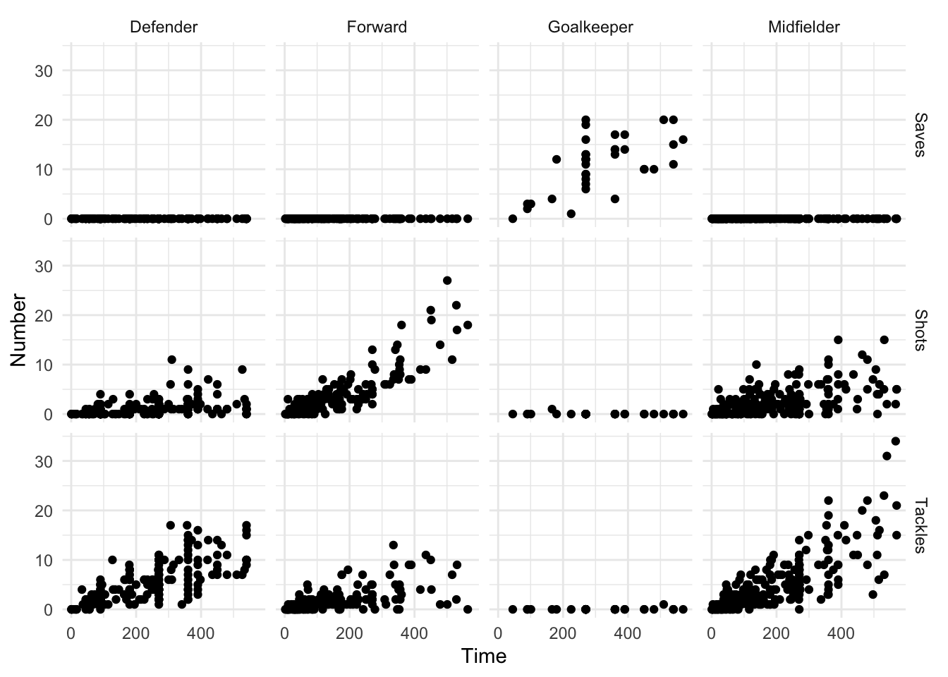
Figure 8.2: Example of a faceted plot created by taking advantage of the pivot_longer function to pull together data.
The pivot_wider function is less commonly needed to tidy data. It can, however, be useful for creating summary tables. For example, if you wanted to print a table of the average number and range of passes by position for the top four teams in this World Cup (Spain, Netherlands, Uruguay, and Germany), you could run:
library(knitr)

# Summarize the data to create the summary statistics you want
wc_table <- worldcup %>%
  filter(Team %in% c("Spain", "Netherlands", "Uruguay", "Germany")) %>%
  select(Team, Position, Passes) %>%
  group_by(Team, Position) %>%
  summarize(ave_passes = mean(Passes),
            min_passes = min(Passes),
            max_passes = max(Passes),
            pass_summary = paste0(round(ave_passes), " (",
                                  min_passes, ", ",
                                  max_passes, ")"),
            .groups = "drop") %>%
  select(Team, Position, pass_summary)
# What the data looks like before using `pivot_wider`
wc_table
## # A tibble: 16 x 3
## Team Position pass_summary
## <fct> <fct> <chr>
## 1 Germany Defender 190 (44, 360)
## 2 Germany Forward 90 (5, 217)
## 3 Germany Goalkeeper 99 (99, 99)
## 4 Germany Midfielder 177 (6, 423)
## 5 Netherlands Defender 182 (30, 271)
## 6 Netherlands Forward 97 (12, 248)
## 7 Netherlands Goalkeeper 149 (149, 149)
## 8 Netherlands Midfielder 170 (22, 307)
## 9 Spain Defender 213 (1, 402)
## 10 Spain Forward 77 (12, 169)
## 11 Spain Goalkeeper 67 (67, 67)
## 12 Spain Midfielder 212 (16, 563)
## 13 Uruguay Defender 83 (22, 141)
## 14 Uruguay Forward 100 (5, 202)
## 15 Uruguay Goalkeeper 75 (75, 75)
## 16 Uruguay Midfielder 100 (1, 252)# Use pivot_wider to create a prettier format for a table
wc_table %>%
pivot_wider(names_from = "Position",
values_from = "pass_summary") %>%
kable()| Team | Defender | Forward | Goalkeeper | Midfielder |
|---|---|---|---|---|
| Germany | 190 (44, 360) | 90 (5, 217) | 99 (99, 99) | 177 (6, 423) |
| Netherlands | 182 (30, 271) | 97 (12, 248) | 149 (149, 149) | 170 (22, 307) |
| Spain | 213 (1, 402) | 77 (12, 169) | 67 (67, 67) | 212 (16, 563) |
| Uruguay | 83 (22, 141) | 100 (5, 202) | 75 (75, 75) | 100 (1, 252) |
Notice in this example how pivot_wider has been used at the very end of the code sequence to convert the summarized data into a shape that offers a better tabular presentation for a report. In the pivot_wider call, you first specify the name of the column to use for the new column names (Position in this example) and then specify the column to use for the cell values (pass_summary here).
In this code, I’ve used the kable function from the knitr package to create the summary table in a table format, rather than as basic R output. This function is very useful for formatting basic tables in R markdown documents. For more complex tables, check out the pander and xtable packages.