17 HOMEWORK 2 [DUE 10/9]
DUE: 10/9
The goal of this assignment is to get used to designing and writing functions. Writing functions involves thinking about how code should be divided up and what the interface/arguments should be. In addition, you need to think about what the function will return as output.
17.1 Homework Submission
Please write up your homework as an R markdown document processed with knitr. Compile your document as an HTML file submit your HTML file to the dropbox on CoursePlus. Please show all your code (i.e. make sure to set echo = TRUE) for each of the answers to the three parts.
17.2 Part 1
The exponential of a number can be written as an infinite series expansion of the form \[ \exp(x) = 1 + x + \frac{x^2}{2!} + \frac{x^3}{3!} + \cdots \] Of course, we cannot compute an infinite series by the end of this term and so we must truncate it at a certain point in the series. The truncated sum of terms represents an approximation to the true exponential, but the approximation may be usable.
Write a function that computes the exponential of a number using the truncated series expansion. The function should take two arguments:
x: the number to be exponentiatedk: the number of terms to be used in the series expansion beyond the constant 1. The value ofkis always \(\geq 1\).
For example, if \(k = 1\), then the Exp function should return the number \(1 + x\). If \(k = 2\), then you should return the number \(1 + x + x^2/2!\).
You can assume that the input value
xwill always be a single number.You can assume that the value
kwill always be an integer \(\geq 1\).Do not use the
exp()function in R.The
factorial()function can be used to compute factorials.
Your function should produce output like the following:
17.3 Part 2
The data for this part come from a study of indoor air pollution and respiratory disease conducted here at Johns Hopkins. A high-resolution air pollution monitor was placed in each home to collect continuous levels of particulate matter over the period of a few days (each measurement represents a 5-minute average). In addition, measurements were taken in different rooms of the house as well as on multiple visits.
Initially, we’d like to explore the data for each subject (indicated by the id column) and so we can make some exploratory time series plots of the data.
The following code plots the data from one subject (id == 2) on the baseline visit (visit == 0) and in the bedroom (room == "bedroom").
library(tidyverse)
mie <- read_csv("data/MIE.csv.gz", col_types = "iicdi")
mie %>%
        filter(id == 20 & visit == 0 & room == "bedroom") %>%
        ggplot(aes(timepoint, value)) +
        geom_line() +
        theme_minimal()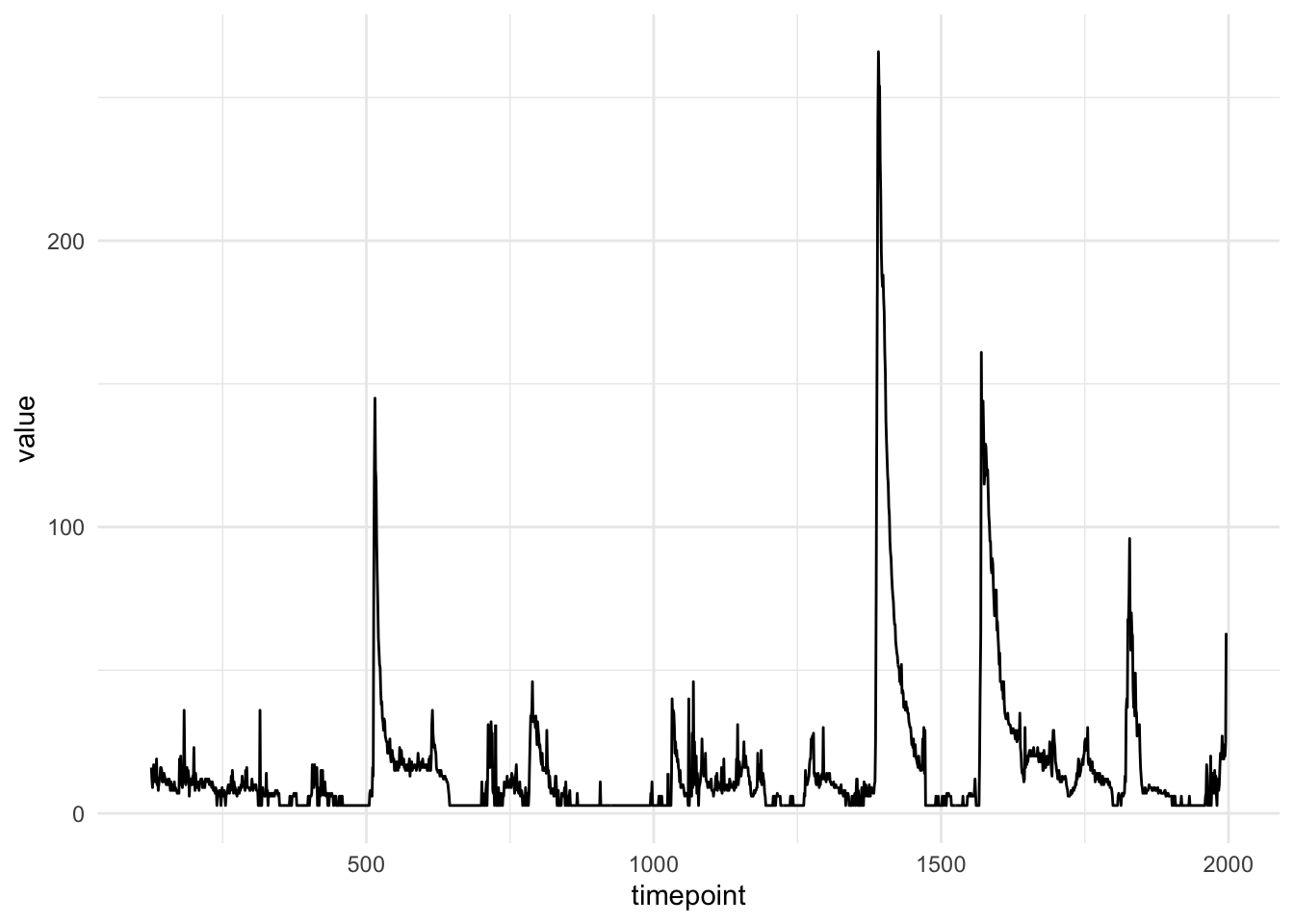
While this code is useful, it only provides us information on one subject, on one visit, in one room. We could cut and paste this code to look at other subjects/visits/rooms, but that can be error prone and just plain messy.
The aim here is to design and implement a function that can be re-used to visualize all of the data in this dataset.
There are 3 aspects that may vary in the dataset: The id, the visit, and the room. Note that not all combinations of id, visit, and room have measurements.
Your function should take as input one of the 3 possible factors. You need to decide which one of those it will be. You do NOT need to write separate functions for all three variables. For example, if you choose to use id as an input, you do not need separate functions for visit or room.
Given the input from the user, your function should present all of the data for that input. For example, if the input is
id = 2, then you should plot the data for all rooms and all visits. If you the input isvisit = 0, then you should plot data for all ids and all rooms, etc. It should be possible visualize the entire dataset with your function (through repeated calls to your function).Your function should produce a single plot that contains all the data. Furthermore, the data should be readable on that plot so that it is in fact useful. You will likely want to use multiple panels/facets, colors, symbols, line types, etc. to enhance the readability of your plot.
If the user enters an input that does not exist in the dataset, your function should catch that and report an error (via the
stop()function).
For your homework submission
Write a short description of how you chose to design your function and why.
Present the code for your function in the R markdown document.
Include at least one example of output from your function.
17.4 Part 3
For this part you will write a few functions that simulate the process of conducting a study of particulate matter in children’s homes. The vector pm contains simulated particulate matter measurements in the homes of 5000 children in an school district. (NOTE: The code for simulating the pm vector is contained in Part B.)
Suppose as an investigator, you want to survey the homes of the students in an elementary school to measure the indoor particulate matter. You only have funding to survey 20 homes, but you want to estimate the average pm concentration in the homes of children from this school with a confidence interval.
Part A
First, write a function called calculate_CI95 that:
Takes as input a vector of data, and samples 20 values from that vector. Try looking at the documentation for the function
sample(). Note that you will sample without replacement here.Calculates an average particulate matter concentration for the 20 students sampled.
Calculates a 95% confidence interval for the average particulate matter in the population. If you have never calculated a confidence interval, the confidence interval consists of a lower bound
mean(x) - 1.96 * sd(x)/sqrt(20)and upper boundmean(x) + 1.96 * sd(x)/sqrt(20).Returns a named vector of length 3, where the first value is the lower bound, the second value is the mean, and the third value is the upper bound.
Part B
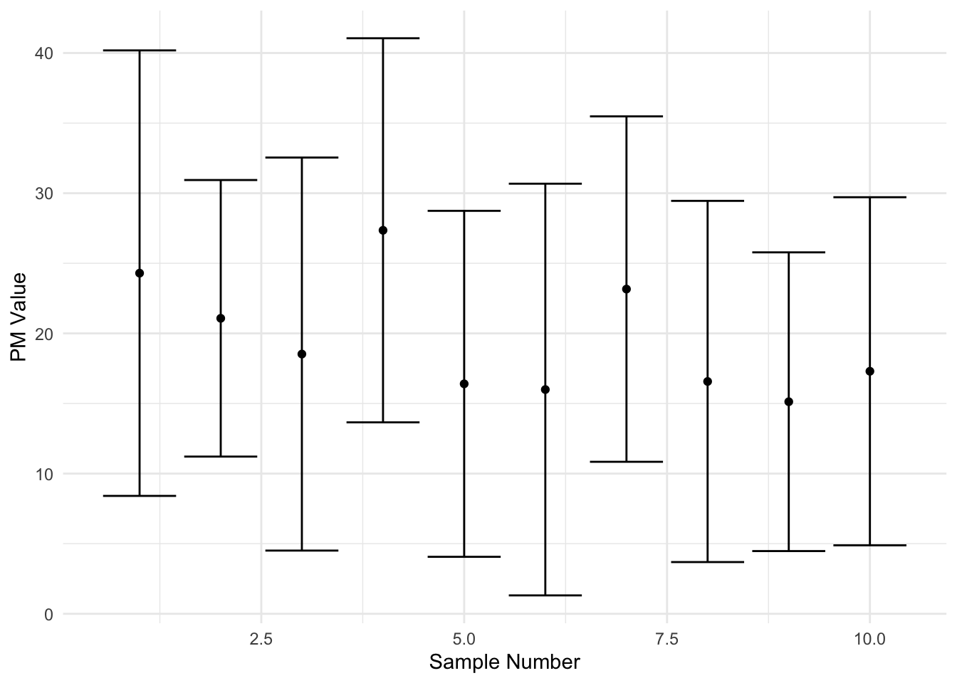
Second, write a function called plot_simulationCI that can simulate the process of conducting this study many times. Your function should have the arguments n, the number of studies to be replicated, and data, the vector of data to simulate draws from. In particular your function will:
Use the function
replicate()along withcalculate_CI95()to make means and confidence intervals fornrandom draws from the population. You may also implement this as aforloop if you wish.Plots all
nconfidence intervals on the same plot. Think about usingggplot()with bothgeom_point()for the means andgeom_errorbar()for the lower and upper bounds of the confidence interval.
Finally, run both functions on the vector ‘pm’ generated with the code below to print a sample confidence interval (part A) and sample plot with 10 confidence intervals (part B).
The following code should be used to simulate the data for this problem.
set.seed(1000)
pm <- c(exp(rnorm(2000, mean = 3, sd = 1)),
        exp(rnorm(2000, mean = 1, sd = 1.5)),
        exp(rnorm(1000, mean = .5, sd = 1)))
ggplot() +
        geom_histogram(aes(x = pm), bins = 10)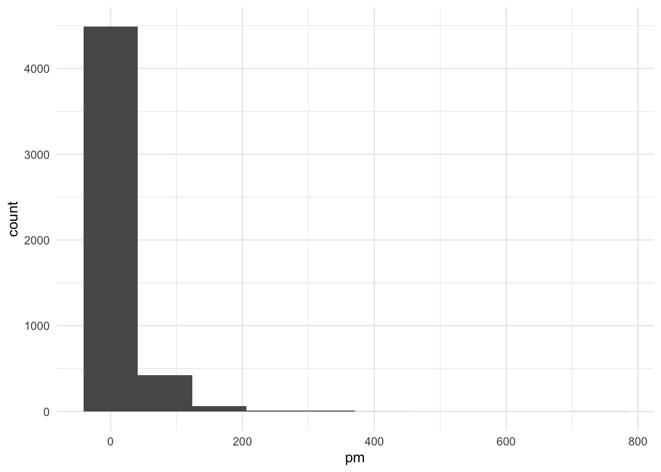
Here is a sample of what the output should look like.
And here is a sample of what the plot should look like.