4.7 Building New Graphical Elements
Some of the key elements of a data graphic made with ggplot2 are geoms and stats. The fact is, the ggplot2 package comes with tremendous capabilities that allow users to make a wide range of interesting and rich data graphics. These graphics can be made through a combination of calls to various geom_* and stat_* functions (as well as other classes of functions).
So why would one want to build a new geom or stat on top of all that ggplot2 already provides?
There are two key reasons for building new geoms and stats for ggplot2:
Implement a new feature. There may be something very specific to your application that is not yet implemented—a new statistical modeling approach or a novel plotting symbol. In this case you don’t have much choice and need to extend the functionality of
ggplot2.Simplify a complex workflow. With certain types of analyses you may find yourself producing the same kind of plot elements repeatedly. These elements may involve a combination of points, lines, facets, or text and essentially encapsulate a single idea. In that case it may make sense to develop a new geom to literally encapsulate the collection of plot elements and to make it simpler to include these things in your future plots.
Building new stats and geoms is the plotting equivalent of writing functions (that may sound a little weird because stats and geoms are functions, but they are thought of a little differently from generic functions). While the action taken by a function can typically be executed using separate expressions outside of a function context, it is often convenient for the user to encapsulate those actions into a clean function. In addition, writing a function allows you to easily parameterize certain elements of that code. Creating new geoms and stats similarly allows for a simplification of code and for allowing users to easily tweak certain elements of a plot without having to wade through an entire mess of code every time.
4.7.1 Building a Geom
New geoms in ggplot2 inherit from a top level class called Geom and are constructed using a two step process.
The
ggproto()function is used to construct a new class corresponding to your new geom. This new class specifies a number of attributes and functions that describe how data should be drawn on a plot.The
geom_*function is constructed as a regular function. This function returns a layer to that can be added to a plot created with theggplot()function.
The basic setup for a new geom class will look something like the following.
GeomNEW <- ggproto("GeomNEW", Geom,
        required_aes = <a character vector of required aesthetics>,
        default_aes = aes(<default values for certain aesthetics>),
        draw_key = <a function used to draw the key in the legend>,
        draw_panel = function(data, panel_scales, coord) {
                ## Function that returns a grid grob that will
                ## be plotted (this is where the real work occurs)
        }
)
The ggproto function is used to create the new class. Here, “NEW” will be replaced by whatever name you come up with that best describes what your new geom is adding to a plot. The four things listed inside the class are required of all geoms and must be specified.
The required aesthetics should be straightforward—if your new geom makes a special kind of scatterplot, for example, you will likely need x and y aesthetics. Default values for aesthetics can include things like the plot symbol (i.e. shape) or the color.
Implementing the draw_panel function is the hard part of creating a new geom. Here you must have some knowledge of the grid package in order to access the underlying elements of a ggplot2 plot, which based on the grid system. However, you can implement a reasonable amount of things with knowledge of just a few elements of grid.
The draw_panel function has three arguments to it. The data element is a data frame containing one column for each aesthetic specified, panel_scales is a list containing information about the x and y scales for the current panel, and coord is an object that describes the coordinate system of your plot.
The coord and the panel_scales objects are not of much use except that they transform the data so that you can plot them.
library(grid)
GeomMyPoint <- ggproto("GeomMyPoint", Geom,
        required_aes = c("x", "y"),
        default_aes = aes(shape = 1),
        draw_key = draw_key_point,
        draw_panel = function(data, panel_scales, coord) {
                ## Transform the data first
                coords <- coord$transform(data, panel_scales)

                ## Let's print out the structure of the 'coords' object
                str(coords)

                ## Construct a grid grob
                pointsGrob(
                        x = coords$x,
                        y = coords$y,
                        pch = coords$shape
                )
        })
I> In this example we print out the structure of the coords object with the str() function just so you can see what is in it. Normally, when building a new geom you wouldn’t do this.
In addition to creating a new Geom class, you need to create the actually function that will build a layer based on your geom specification. Here, we call that new function geom_mypoint(), which is modeled after the built in geom_point() function.
geom_mypoint <- function(mapping = NULL, data = NULL, stat = "identity",
                         position = "identity", na.rm = FALSE,
                         show.legend = NA, inherit.aes = TRUE, ...) {
        ggplot2::layer(
                geom = GeomMyPoint, mapping = mapping,
                data = data, stat = stat, position = position,
                show.legend = show.legend, inherit.aes = inherit.aes,
                params = list(na.rm = na.rm, ...)
        )
}
Now we can use our new geom on the worldcup dataset.
ggplot(data = worldcup, aes(Time, Shots)) + geom_mypoint()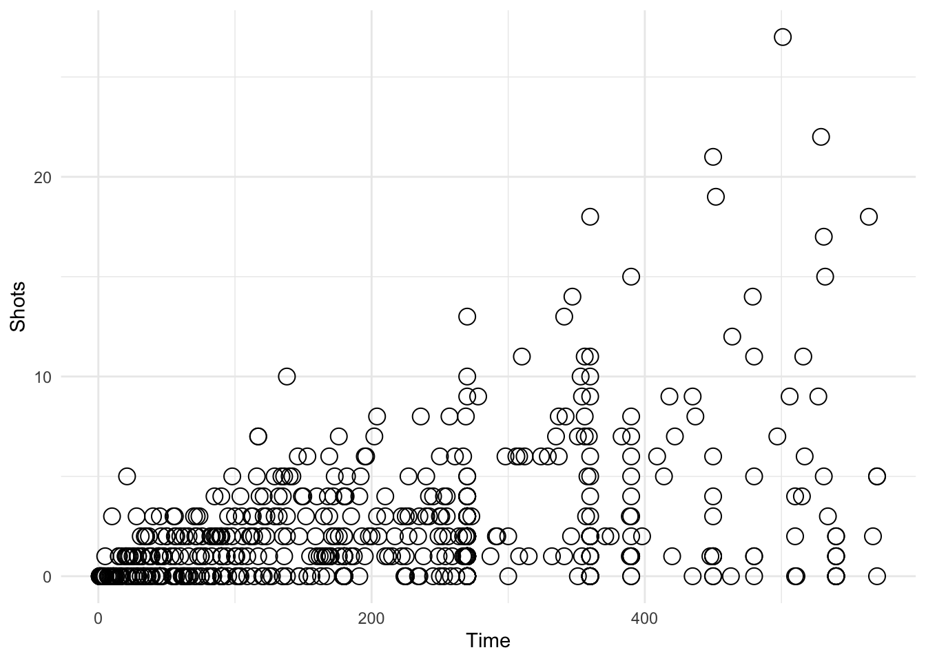
Figure 4.118: Using a custom geom
'data.frame':   595 obs. of  5 variables:
 $ x    : num  0.0694 0.6046 0.3314 0.4752 0.1174 ...
 $ y    : num  0.0455 0.0455 0.0455 0.0791 0.1128 ...
 $ PANEL: Factor w/ 1 level "1": 1 1 1 1 1 1 1 1 1 1 ...
 $ group: int  -1 -1 -1 -1 -1 -1 -1 -1 -1 -1 ...
 $ shape: num  1 1 1 1 1 1 1 1 1 1 ...
From the str() output we can see that the coords object contains the x and y aesthetics, as well as the shape aesthetic that we specified as the default. Note that both x and y have been rescaled to be between 0 and 1. This is the normalized parent coordinate system.
4.7.2 Example: An Automatic Transparency Geom
One problem when making scatterplots of large amounts of data is overplotting. In particular, with ggplot2’s default solid circle as the plotting shape, if there are many overlapping points all you will see is a solid mass of black.
One solution to this problem of overplotting is to make the individual points transparent by setting the alpha channel. The alpha channel is a number between 0 and 1 where 0 is totally transparent and 1 is completely opaque. With transparency, if two points overlap each other, they will be darker than a single point sitting by itself. Therefore, you can see more of the “density” of the data when the points are transparent.
The one requirement for using transparency in scatterplots is computing the amount of transparency, or the the alpha channel. Often this will depend on the number of points in the plot. For a simple plot with a few points, no transparency is needed. For a plot with hundreds or thousands of points, transparency is required. Computing the exact amount of transparency may require some experimentation.
The following example creates a geom that computes the alpha channel based on the number of points that are being plotted. First we create the Geom class, which we call GeomAutoTransparent. This class sets the alpha aesthetic to be 0.3 if the number of data points is between 100 and 200 and 0.15 if the number of data points is over 200. If the number of data points is 100 or less, no transparency is used.
GeomAutoTransparent <- ggproto("GeomAutoTransparent", Geom,
        required_aes = c("x", "y"),
        default_aes = aes(shape = 19),
        draw_key = draw_key_point,
        draw_panel = function(data, panel_scales, coord) {
                ## Transform the data first
                coords <- coord$transform(data, panel_scales)

                ## Compute the alpha transparency factor based on the
                ## number of data points being plotted
                n <- nrow(data)
                if(n > 100 && n <= 200)
                        coords$alpha <- 0.3
                else if(n > 200)
                        coords$alpha <- 0.15
                else
                        coords$alpha <- 1
                ## Construct a grid grob
                grid::pointsGrob(
                        x = coords$x,
                        y = coords$y,
                        pch = coords$shape,
                        gp = grid::gpar(alpha = coords$alpha)
                )
        })
Now we need to create the corresponding geom function, which we slightly modify from geom_point(). Note that the geom argument to the layer() function takes our new GeomAutoTransparent class as its argument.
geom_transparent <- function(mapping = NULL, data = NULL, stat = "identity",
                         position = "identity", na.rm = FALSE,
                         show.legend = NA, inherit.aes = TRUE, ...) {
        ggplot2::layer(
                geom = GeomAutoTransparent, mapping = mapping,
                data = data, stat = stat, position = position,
                show.legend = show.legend, inherit.aes = inherit.aes,
                params = list(na.rm = na.rm, ...)
        )
}
Now we can try out our new geom_transparent() function with differing amounts of data to see how the transparency works. Here is the entire worldcup dataset, which has 595 observations.
ggplot(data = worldcup, aes(Time, Shots)) + geom_transparent()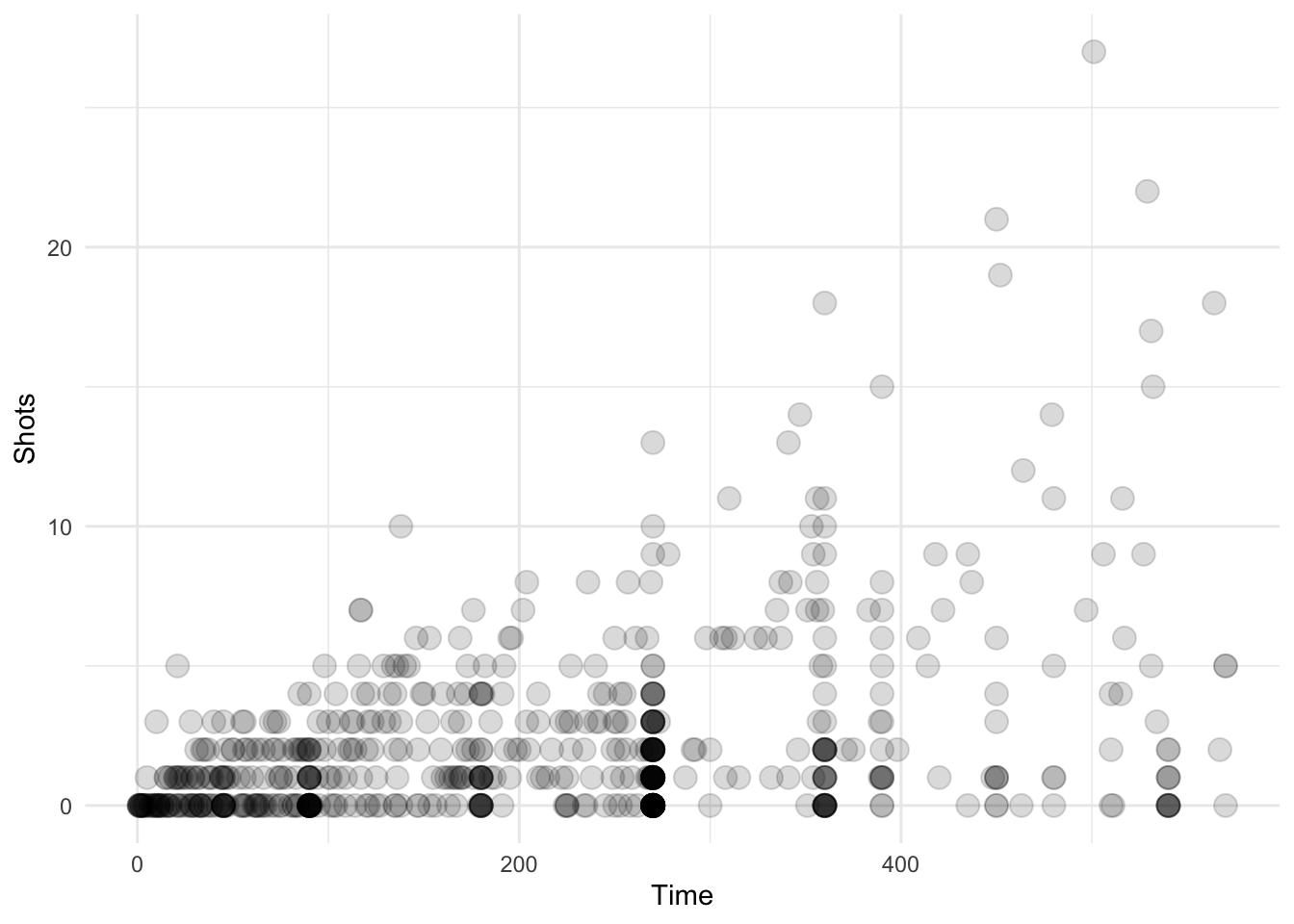
Figure 4.119: Scatterplot with auto transparency geom
Here we take a random sample of 150 observations. The transparency should be a little less in this plot.
library(dplyr)
ggplot(data = sample_n(worldcup, 150), aes(Time, Shots)) +
        geom_transparent()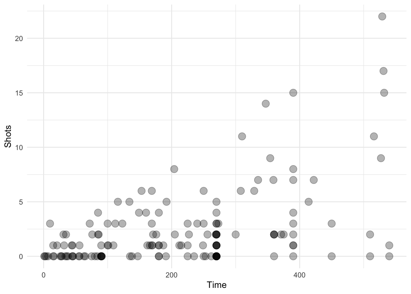
Figure 4.120: Scatterplot with auto transparency geom
Here we take a random sample of 50 observations. There should be no transparency used in this plot.
ggplot(data = sample_n(worldcup, 50), aes(Time, Shots)) +
        geom_transparent()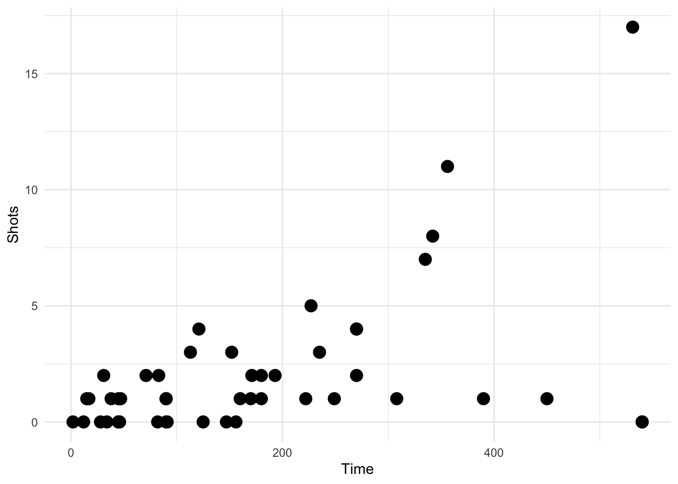
Figure 4.121: Scatterplot with auto transparency geom
We can also reproduce a faceted plot from the previous section with our new geom and the features of the geom will propagate to the panels.
ggplot(data = worldcup, aes(Time, Shots)) +
        geom_transparent() +
        facet_wrap(~ Position, ncol = 2) +
        newtheme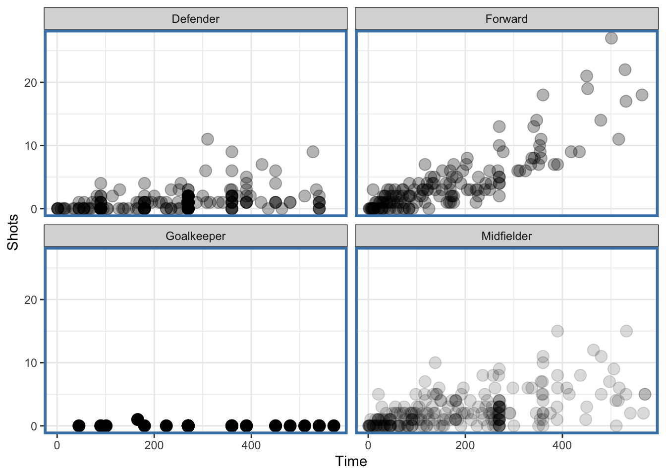
Figure 4.122: Faceted plot with auto transparency geom
Notice that the data for the “Midfielder,” “Defender,” and “Forward” panels have some transparency because there are more points there but the “Goalkeeper” panel has no transparency because it has relatively few points.
It’s worth noting that in this example, a different approach might have been to not create a new geom, but rather to compute an “alpha” column in the dataset that was a function of the number of data points (or the number of data points in each subgroup). Then you could have just set the alpha aesthetic to be equal to that column and ggplot2 would have naturally mapped the appropriate alpha value to the the right subgroup. However, there a few issues with that approach:
It involves adding a column to the data that isn’t fundamentally related to the data (it is related to presenting the data); and
Some version of that alpha computation would need to be done every time you plotted the data in a different way. For example if you faceted on a different grouping variable, you’d need to compute the alpha value based on the number of points in the new subgroups.
The advantage of creating a geom in this case is that it abstracts the computation, removes the need to modify the data each time, and allows for a simpler communication of what is trying to be done in this plotting code.
4.7.3 Building a Stat
In addition to geoms, we can also build a new stat in ggplot2, which can be used to abstract out any computation that may be needed in the creation/drawing of a geom on a plot. Separating out any complex computation that may be needed by a geom can simplify the writing of the geom down the road.
Building a stat looks a bit like building a geom but there are different functions and classes that need to be specified. Analogous to creating a geom, we need to use the ggproto() function to create a new class that will usually inhert from the Stat class. Then we will need to specify a stat_* function that will create the layer that will be used by ggplot2 and related geom_* functions.
The template for building a stat will look something like the following:
StatNEW <- ggproto("StatNEW", Stat,
                   compute_group = <a function that does computations>,
                   default_aes = aes(<default values for certain aesthetics>),
                   required_aes = <a character vector of required aesthetics>)
The ggproto() function is used to create the new class and “NEW”" will be replaced by whatever name you come up with that best describes what your new stat is computing.
The ultimate goal of a stat is to render the data in some way to make it suitable for plotting. To that end, the compute_group() function must return a data frame so that the plotting machinery in ggplot2 (which typically expects data frames) will know what to do.
If the output of your stat can be used as input to a standard/pre-existing geom, then there is no need to write a custom geom to go along with your stat. Your stat only needs format its output in a manner that existing geoms will recognize. For example, if you want to render the data in a special way, but ultimately plot them as polygons, you may be able to take advantage of the existing geom_polygon() function.
4.7.4 Example: Normal Confidence Intervals
One task that is common in the course of data analysis or statistical modeling is plotting a set of parameter estimates along with a 95% confidence interval around those points. Given an estimate and a standard error, basic statistical theory says that we can approximate a 95% confidence interval for the parameter by taking the estimate and adding/subtracting 1.96 times the standard error. We can build a simple stat that takes an estimate and standard error and constructs the data that would be needed by geom_segment() in order to draw the approximate 95% confidence intervals.
Let’s take the airquality dataset that comes with R and compute the monthly mean levels of ozone along with standard errors for those monthly means.
library(datasets)
library(dplyr)
data("airquality")
monthly <- dplyr::group_by(airquality, Month) %>%
        dplyr::summarize(ozone = mean(Ozone, na.rm = TRUE),
                  stderr = sd(Ozone, na.rm = TRUE) / sqrt(sum(!is.na(Ozone))))
monthly
# A tibble: 5 x 3
  Month ozone stderr
  <int> <dbl>  <dbl>
1     5  23.6   4.36
2     6  29.4   6.07
3     7  59.1   6.20
4     8  60.0   7.78
5     9  31.4   4.48
A simple plot of the monthly means might look as follows.
ggplot(monthly, aes(x = Month, y = ozone)) +
        geom_point() +
        ylab("Ozone (ppb)")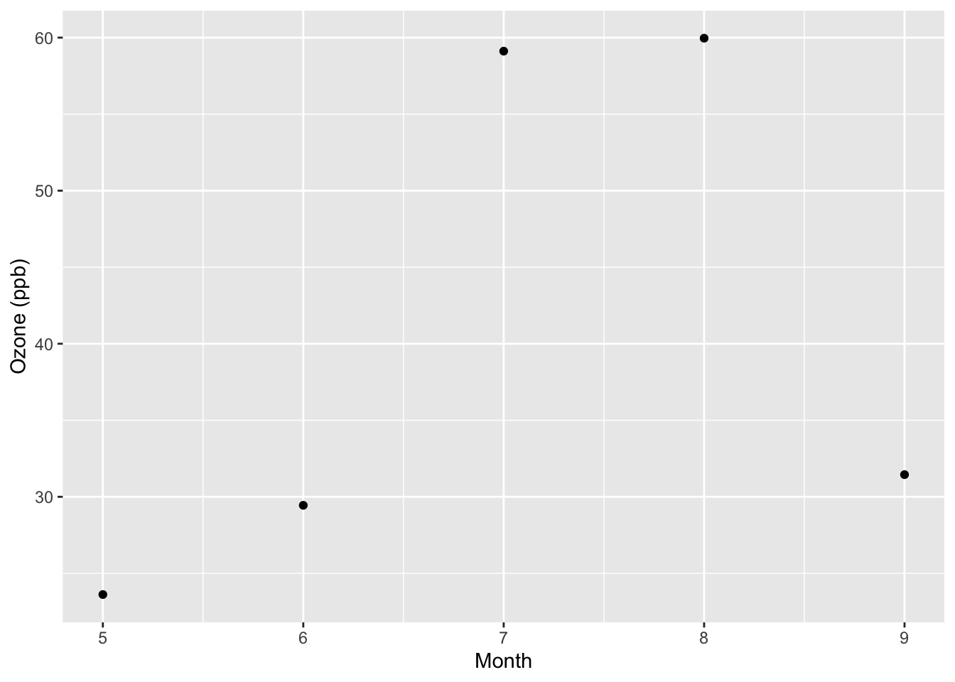
But the above plot does not show the variability we might expect around those monthly means. We can create a stat to do the work for us and feed the information to geom_segment(). First, we need to recall that geom_segment() needs the aesthetics x, xend, y, and yend, which specify the beginning and endpoints of each line segment. Therefore, your stat should also specify this information. The compute_group() function defined within the call to ggproto() should provide this.
StatConfint <- ggproto("StatConfint", Stat,
                       compute_group = function(data, scales) {
                               ## Compute the line segment endpoints
                               x <- data$x
                               xend <- data$x
                               y <- data$y - 1.96 * data$stderr
                               yend <- data$y + 1.96 * data$stderr

                               ## Return a new data frame
                               data.frame(x = x, xend = xend,
                                          y = y, yend = yend)
                       },
                       required_aes = c("x", "y", "stderr")
)
Next we can define a separate stat_* function that builds the layer for ggplot functions.
stat_confint <- function(mapping = NULL, data = NULL, geom = "segment",
                           position = "identity", na.rm = FALSE,
                           show.legend = NA, inherit.aes = TRUE, ...) {
        ggplot2::layer(
                stat = StatConfInt,
                data = data,
                mapping = mapping,
                geom = geom,
                position = position,
                show.legend = show.legend,
                inherit.aes = inherit.aes,
                params = list(na.rm = na.rm, ...)
        )
}
With the new stat we can revise our original plot to include approximate 95% confidence intervals around the monthly means for ozone.
ggplot(data = monthly, aes(x = Month, y = ozone, stderr = stderr)) +
        geom_point() +
        ylab("Ozone (ppb)") +
        geom_segment(stat = "confint")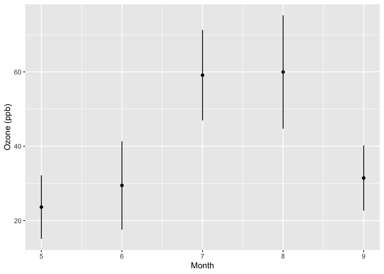
From the new plot we can see that the variability about the mean in August is somewhat greater than it is in July or September.
The advantage writing a separate stat in this case is that it removes the cruft of computing the +/- 1.96 * stderr every time you want to plot the confidence intervals. If you are making these kinds of plots commonly, it can be handy to clean up the code by abstracting the computation into a separate stat_* function.
4.7.5 Combining Geoms and Stats
Combining geoms and stats gives you a way of creating new graphical elements that make use of special computations that you define. In addition, if you require some custom drawing that is not immediately handled by an existing geom, then you may consider writing a separate geom to handle the data computed by your stat. In this section we show how to combine stats with geoms to create a custom plot.
The example we will use is creating a “skinny boxplot,” which looks something like this.
## This code is not runnable yet!
library(ggplot2)
library(datasets)
data(airquality)
mutate(airquality, Month = factor(Month)) %>%
        ggplot(aes(Month, Ozone)) +
        geom_skinnybox()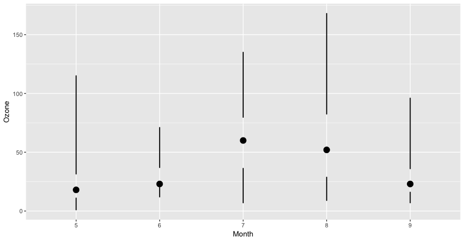
Skinny Boxplot
This boxplot differs from the traditional boxplot (e.g. geom_boxplot()) in the following ways:
- The “whiskers” extend to the minimum and the maximum of the data
- The medians are represented by a point rather than a line
- There is no box indicating the region between the 25th and 75th percentiles
While it’s certainly possible to manipulate existing R functions to create such a plot, doing so would not necessarily make it clear to any reader of the code that this is what you were doing. Also, if you play to make a lot of these kinds of plots, having a dedicated geom can make things a bit more compact and streamlined.
First we can create a stat that computes the relevant summary statistics from the data: minimum, first quartile, median, third quartile, and the maximum.
StatSkinnybox <- ggproto("StatSkinnybox", Stat,
                         compute_group = function(data, scales) {
                                 probs <- c(0, 0.25, 0.5, 0.75, 1)
                                 qq <- quantile(data$y, probs, na.rm = TRUE)
                                 out <- qq %>% as.list %>% data.frame
                                 names(out) <- c("ymin", "lower", "middle",
                                                 "upper", "ymax")
                                 out$x <- data$x[1]
                                 out
                         },
                         required_aes = c("x", "y")
                         )

stat_skinnybox <- function(mapping = NULL, data = NULL, geom = "skinnybox",
                           position = "identity", show.legend = NA,
                           outliers = TRUE, inherit.aes = TRUE, ...) {
        ggplot2::layer(
                stat = StatSkinnybox,
                data = data,
                mapping = mapping,
                geom = geom,
                position = position,
                show.legend = show.legend,
                inherit.aes = inherit.aes,
                params = list(outliers = outliers, ...)
        )
}
With the stat available to process the data, we can move on to writing the geom. This set of functions is responsible for drawing the appropriate graphics in the plot region. First we can create the GeomSkinnybox class with the ggproto() function. In that the critical function is the draw_panel() function, which we implement separately because of its length. Note that in the draw_panel_function() function, we need to manually rescale the “lower,” “upper,” and “middle” portions of the boxplot or else they will not appear on the plot (they will be in the wrong units).
library(scales)
draw_panel_function <- function(data, panel_scales, coord) {
        coords <- coord$transform(data, panel_scales) %>%
                mutate(lower = rescale(lower, from = panel_scales$y.range),
                       upper = rescale(upper, from = panel_scales$y.range),
                       middle = rescale(middle, from = panel_scales$y.range))
        med <- pointsGrob(x = coords$x,
                          y = coords$middle,
                          pch = coords$shape)
        lower <- segmentsGrob(x0 = coords$x,
                              x1 = coords$x,
                              y0 = coords$ymin,
                              y1 = coords$lower,
                              gp = gpar(lwd = coords$size))
        upper <- segmentsGrob(x0 = coords$x,
                              x1 = coords$x,
                              y0 = coords$upper,
                              y1 = coords$ymax,
                              gp = gpar(lwd = coords$size))
        gTree(children = gList(med, lower, upper))
}

GeomSkinnybox <- ggproto("GeomSkinnybox", Geom,
                         required_aes = c("x", "ymin", "lower", "middle",
                                          "upper", "ymax"),
                         default_aes = aes(shape = 19, lwd = 2),
                         draw_key = draw_key_point,
                         draw_panel = draw_panel_function
                         )
Finally, we have the actual geom_skinnybox() function, which draws from the stat_skinnybox() function and the GeomSkinnybox class.
geom_skinnybox <- function(mapping = NULL, data = NULL, stat = "skinnybox",
                           position = "identity", show.legend = NA,
                           na.rm = FALSE, inherit.aes = TRUE, ...) {
        layer(
                data = data,
                mapping = mapping,
                stat = stat,
                geom = GeomSkinnybox,
                position = position,
                show.legend = show.legend,
                inherit.aes = inherit.aes,
                params = list(na.rm = na.rm, ...)
        )
}
Now we can actually run the code presented above and make our “skinny” boxplot.
mutate(airquality, Month = factor(Month)) %>%
        ggplot(aes(Month, Ozone)) +
        geom_skinnybox()
4.7.6 Summary
Building new geoms can be a useful way to implement a completely new graphical procedure or to simplify a complex graphical task that must be used repeatedly in many plots. Building a new geom requires defining a new Geom class via ggproto() and defining a new geom_* function that builds a layer based on the new Geom class.
Some further resources that are worth investigating if you are interested in building new graphical elements are
- R Graphics by Paul Murrell, describes the grid graphical system on which
ggplot2is based.