2.7 Profiling and Benchmarking
The learning objectives of this section are:
- Apply profiling and timing tools to optimize R code
Some of the R code that you write will be slow. Slow code often isn’t worth fixing in a script that you will only evaluate a few times, as the time it will take to optimize the code will probably exceed the time it takes the computer to run it. However, if you are writing functions that will be used repeatedly, it is often worthwhile to identify slow sections of the code so you can try to improve speed in those sections.
In this section, we will introduce the basics of profiling R code, using functions from two packages, microbenchmark and profvis. The profvis package is fairly new and requires recent versions of both R (version 3.0 or higher) and RStudio. If you are having problems running either package, you should try updating both R and RStudio (the Preview version of RStudio, which will provide full functionality for profvis, is available for download here).
2.7.1 microbenchmark
The microbenchmark package is useful for running small sections of code to assess performance, as well as for comparing the speed of several functions that do the same thing. The microbenchmark function from this package will run code multiple times (100 times is the default) and provide summary statistics describing how long the code took to run across those iterations. The process of timing a function takes a certain amount of time itself. The microbenchmark function adjusts for this overhead time by running a certain number of “warm-up” iterations before running the iterations used to time the code.
You can use the times argument in microbenchmark to customize how many iterations are used. For example, if you are working with a function that is a bit slow, you might want to run the code fewer times when benchmarking (although with slower or more complex code, it likely will make more sense to use a different tool for profiling, like profvis).
You can include multiple lines of code within a single call to microbenchmark. However, to get separate benchmarks of line of code, you must separate each line by a comma:
library(microbenchmark)
microbenchmark(a <- rnorm(1000),
               b <- mean(rnorm(1000)))
Unit: microseconds
                   expr    min     lq     mean  median     uq    max neval
       a <- rnorm(1000) 59.759 61.946 65.77382 65.9475 69.030 80.450   100
 b <- mean(rnorm(1000)) 63.801 65.706 70.56654 69.5850 74.842 89.362   100
The microbenchmark function is particularly useful for comparing functions that take the same inputs and return the same outputs. As an example, say we need a function that can identify days that meet two conditions: (1) the temperature equals or exceeds a threshold temperature (27 degrees Celsius in the examples) and (2) the temperature equals or exceeds the hottest temperature in the data before that day. We are aiming for a function that can input a data frame that includes a column named temp with daily mean temperature in Celsius, like this data frame:
date          temp
2015-07-01    26.5
2015-07-02    27.2
2015-07-03    28.0
2015-07-04    26.9
2015-07-05    27.5
2015-07-06    25.9
2015-07-07    28.0
2015-07-08    28.2
and outputs a data frame that has an additional binary record_temp column, specifying if that day meet the two conditions, like this:
date          temp    record_temp
2015-07-01    26.5    FALSE
2015-07-02    27.2    TRUE
2015-07-03    28.0    TRUE
2015-07-04    26.9    FALSE
2015-07-05    27.5    FALSE
2015-07-06    25.9    FALSE
2015-07-07    28.0    TRUE
2015-07-08    28.2    TRUE
Below are two example functions that can perform these actions. Since the record_temp column depends on temperatures up to that day, one option is to use a loop to create this value. The first function takes this approach. The second function instead uses tidyverse functions to perform the same tasks.
# Function that uses a loop
find_records_1 <- function(datafr, threshold){
  highest_temp <- c()
  record_temp <- c()
  for(i in 1:nrow(datafr)){
    highest_temp <- max(highest_temp, datafr$temp[i])
    record_temp[i] <- datafr$temp[i] >= threshold &
      datafr$temp[i] >= highest_temp
  }
  datafr <- cbind(datafr, record_temp)
  return(datafr)
}

# Function that uses tidyverse functions
find_records_2 <- function(datafr, threshold){
  datafr <- datafr %>%
    mutate_(over_threshold = ~ temp >= threshold,
            cummax_temp = ~ temp == cummax(temp),
            record_temp = ~ over_threshold & cummax_temp) %>%
    select_(.dots = c("-over_threshold", "-cummax_temp"))
  return(as.data.frame(datafr))
}
If you apply the two functions to the small example data set, you can see that they both create the desired output:
example_data <- data_frame(date = c("2015-07-01", "2015-07-02",
                                    "2015-07-03", "2015-07-04",
                                    "2015-07-05", "2015-07-06",
                                    "2015-07-07", "2015-07-08"),
                           temp = c(26.5, 27.2, 28.0, 26.9,
                                    27.5, 25.9, 28.0, 28.2))
Warning: `data_frame()` is deprecated as of tibble 1.1.0.
Please use `tibble()` instead.
This warning is displayed once every 8 hours.
Call `lifecycle::last_warnings()` to see where this warning was generated.

(test_1 <- find_records_1(example_data, 27))
        date temp record_temp
1 2015-07-01 26.5       FALSE
2 2015-07-02 27.2        TRUE
3 2015-07-03 28.0        TRUE
4 2015-07-04 26.9       FALSE
5 2015-07-05 27.5       FALSE
6 2015-07-06 25.9       FALSE
7 2015-07-07 28.0        TRUE
8 2015-07-08 28.2        TRUE

(test_2 <- find_records_2(example_data, 27))
Warning: `select_()` is deprecated as of dplyr 0.7.0.
Please use `select()` instead.
This warning is displayed once every 8 hours.
Call `lifecycle::last_warnings()` to see where this warning was generated.
Warning: `mutate_()` is deprecated as of dplyr 0.7.0.
Please use `mutate()` instead.
See vignette('programming') for more help
This warning is displayed once every 8 hours.
Call `lifecycle::last_warnings()` to see where this warning was generated.
        date temp record_temp
1 2015-07-01 26.5       FALSE
2 2015-07-02 27.2        TRUE
3 2015-07-03 28.0        TRUE
4 2015-07-04 26.9       FALSE
5 2015-07-05 27.5       FALSE
6 2015-07-06 25.9       FALSE
7 2015-07-07 28.0        TRUE
8 2015-07-08 28.2        TRUE

all.equal(test_1, test_2)
[1] TRUE
The performance of these two functions can be compared using microbenchmark:
record_temp_perf <- microbenchmark(find_records_1(example_data, 27),
                                   find_records_2(example_data, 27))
record_temp_perf
Unit: microseconds
                             expr      min       lq      mean   median
 find_records_1(example_data, 27)  109.209  129.521  142.0319  139.553
 find_records_2(example_data, 27) 4567.623 4663.668 5394.6744 5075.517
        uq       max neval
  151.5925   266.107   100
 5828.2815 11027.781   100
This output gives summary statistics (min, lq, mean, median, uq, and max) describing the time it took to run the two function over the 100 iterations of each function call. By default, these times are given in a reasonable unit, based on the observed profiling times (units are given in microseconds in this case).
It’s useful to check next to see if the relative performance of the two functions is similar for a bigger data set. The chicagoNMMAPS data set from the dlnm package includes temperature data over 15 years in Chicago, IL. Here are the results when we benchmark the two functions with that data (note, this code takes a minute or two to run):
library(dlnm)
data("chicagoNMMAPS")

record_temp_perf_2 <- microbenchmark(find_records_1(chicagoNMMAPS, 27),
                                     find_records_2(chicagoNMMAPS, 27))
record_temp_perf_2
Unit: milliseconds
                              expr       min        lq      mean    median
 find_records_1(chicagoNMMAPS, 27) 10.736679 11.692736 13.042515 12.516340
 find_records_2(chicagoNMMAPS, 27)  4.217998  4.531123  6.532775  4.891684
        uq       max neval
 13.844831  18.73066   100
  5.534997 137.80639   100
While the function with the loop (find_records_1) performed better with the very small sample data, the function that uses tidyverse functions (find_records_2) performs much, much better with a larger data set.
The microbenchmark function returns an object of the “microbenchmark” class. This class has two methods for plotting results, autoplot.microbenchmark and boxplot.microbenchmark. To use the autoplot method, you will need to have ggplot2 loaded in your R session.
library(ggplot2)
# For small example data
autoplot(record_temp_perf)
Coordinate system already present. Adding new coordinate system, which will replace the existing one.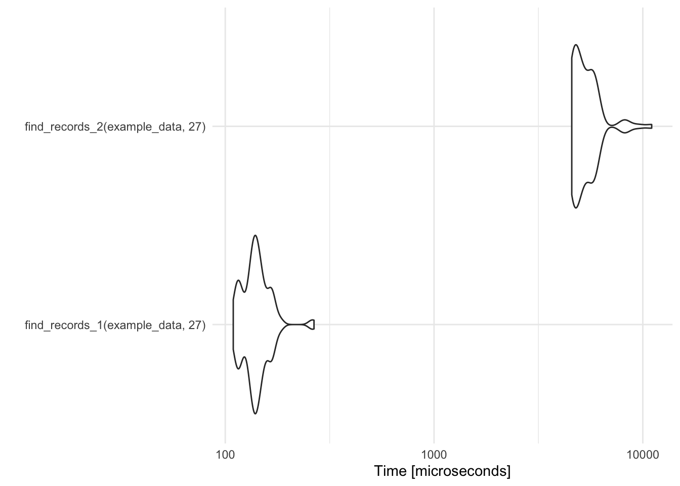
Figure 2.3: Timing comparison of find records functions
# For larger data set
autoplot(record_temp_perf_2)
Coordinate system already present. Adding new coordinate system, which will replace the existing one.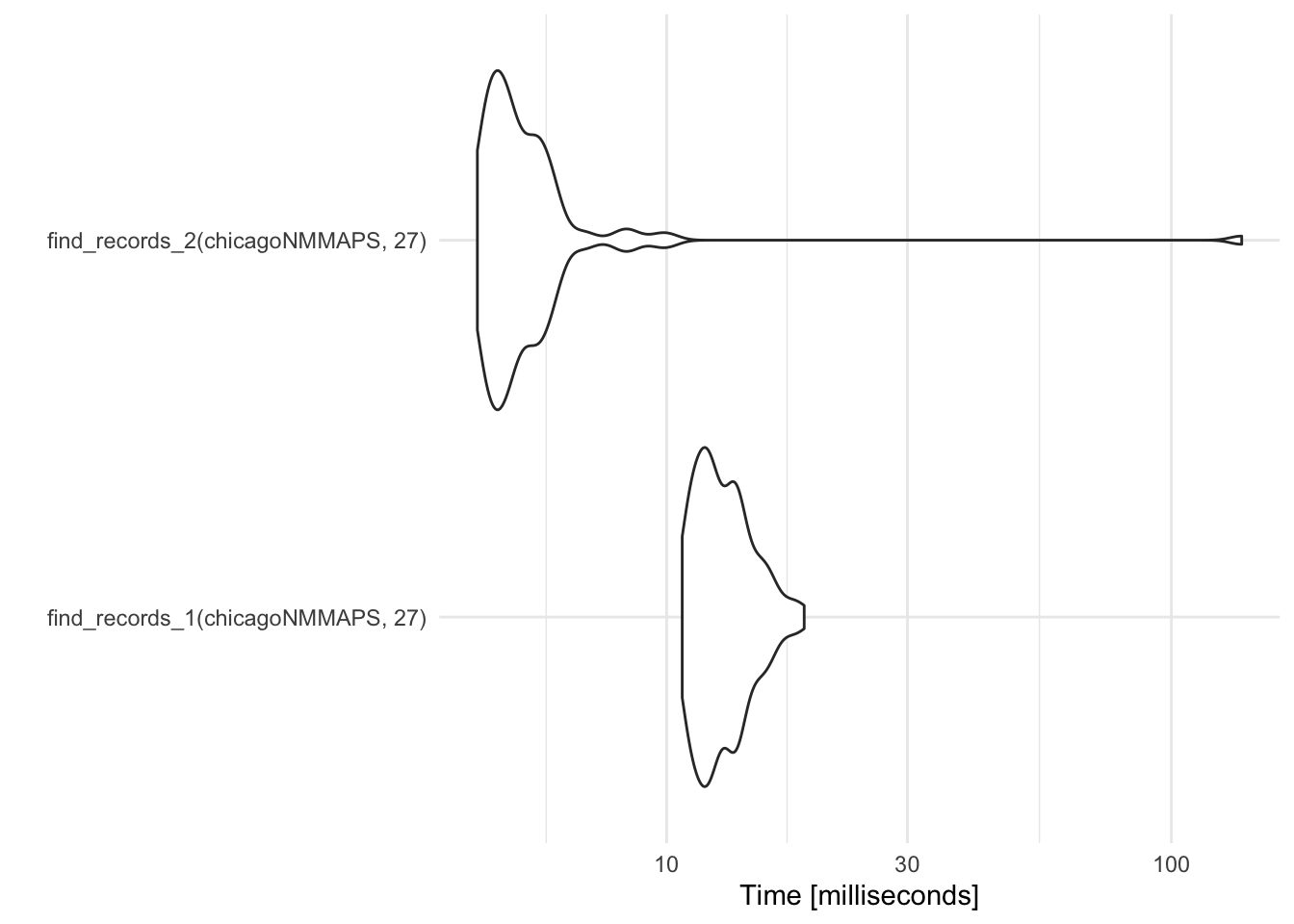
Figure 2.4: Timing comparison of find records functions
By default, this plot gives the “Time” axis on a log scale. You can change this with the argument log = FALSE.
2.7.2 profvis
Once you’ve identified slower code, you’ll likely want to figure out which parts of the code are causing bottlenecks. The profvis function from the profvis package is very useful for this type of profiling. This function uses the RProf function from base R to profile code, and then displays it in an interactive visualization in RStudio. This profiling is done by sampling, with the RProf function writing out the call stack every 10 milliseconds while running the code.
To profile code with profvis, just input the code (in braces if it is mutli-line) into profvis within RStudio. For example, we found that the find_records_1 function was slow when used with a large data set. To profile the code in that function, run:
library(profvis)
datafr <- chicagoNMMAPS
threshold <- 27

profvis({
  highest_temp <- c()
  record_temp <- c()
  for(i in 1:nrow(datafr)){
    highest_temp <- max(highest_temp, datafr$temp[i])
    record_temp[i] <- datafr$temp[i] >= threshold &
      datafr$temp[i] >= highest_temp
  }
  datafr <- cbind(datafr, record_temp)
})
The profvis output gives you two options for visualization: “Flame Graph” or “Data” (a button to toggle between the two is given in the top left of the profvis visualization created when you profile code). The “Data” output defaults to show you the time usage of each first-level function call. Each of these calls can be expanded to show deeper and deeper functions calls within the call stack. This expandable interface allows you to dig down within a call stack to determine what calls are causing big bottlenecks. For functions that are part of a package you have loaded with devtools::load_all, this output includes a column with the file name where a given function is defined. This functionality makes this “Data” output pane particularly useful in profiling functions in a package you are creating.
The “Flame Graph” view in profvis output gives you two panels. The top panel shows the code called, with bars on the right to show memory use and time spent on the line. The bottom panel also visualizes the time used by each line of code, but in this case it shows time use horizontally and shows the full call stack at each time sample, with initial calls shown at the bottom of the graph, and calls deeper in the call stack higher in the graph. Clicking on a block in the bottom panel will show more information about a call, including which file it was called from, how much time it took, how much memory it took, and its depth in the call stack.
Figure ?? shows example output from profiling the code in the find_records_1 function defined earlier in this section.
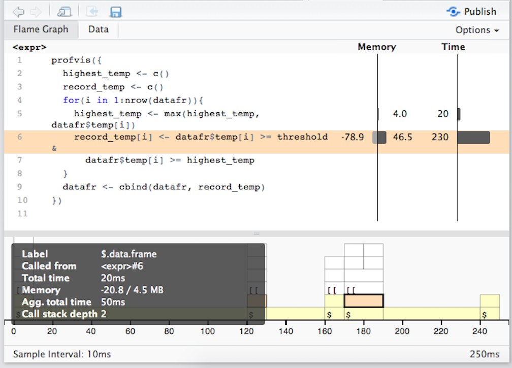
Example of profvis output for a function to find record temperatures.
Based on this visualization, most of the time is spent on line 6, filling in the record_temp vector. Now that we know this, we could try to improve the function, for example by doing a better job of initializing vectors before running the loop.
The profvis visualization can be used to profile code in functions you’re writing as part of a package. If some of the functions in the code you are profiling are in a package currently loaded with loaded with devtools::load_all, the top panel in the Flame Graph output will include the code defining those functions, which allows you to explore speed and memory use within the code for each function. You can also profile code within functions from other packages– for more details on the proper set-up, see the “FAQ” section of RStudio’s profvis documentation.
The profvis function will not be able to profile code that runs to quickly. Trying to profile functions that are too fast will give you the following error message:
Error in parse_rprof(prof_output, expr_source) :
  No parsing data available. Maybe your function was too fast?
You can use the argument interval in profvis to customize the sampling interval. The default is to sample every 10 milliseconds (interval = 0.01), but you can decrease this sampling interval. In some cases, you may be able to use this option to profile faster-running code. However, you should avoid using an interval smaller than about 5 milliseconds, as below that you will get inaccurate estimates with profvis. If you are running very fast code, you’re better off profiling with microbenchmark, which can give accurate estimates at finer time intervals.
Here are some tips for optimizing your use of profvis:
- You may find it convenient to use the “Show in new window” button on the RStudio pane with profiling results to expand this window while you are interpreting results.
- An “Options” button near the top right gives different options for how to display the profiling results, including whether to include memory profiling results and whether to include lines of code with zero time.
- You can click-and-drag results in the bottom visualization panel, as well as pan in and out.
- You may need to update your version of RStudio to be able to use the full functionality of
profvis. You can download a Preview version of RStudio here. - If you’d like to share code profiling results from
profvispublicly, you can do that by using the “Publish” button on the top right of the rendered profile visualization to publish the visualization to RPubs. The “FAQ” section of RStudio’sprofvisdocumentation includes more tips for sharing a code profile visualization online. - If you get a lot of blocks labeled “<Anonymous>,” try updating your version of R. In newer versions of R, functions called using
package::function()syntax orlist$function()syntax are labeled in profiling blocks in a more meaningful way. This is likely to be a particular concern if you are profiling code in a package you are developing, as you will often be usingpackage::function()syntax extensively to pass CRAN checks.
2.7.3 Find out more
If you’d like to learn more about profiling R code, or improving performance of R code once you’ve profiled, you might find these resources helpful:
- RStudio’s
profvisdocumentation - Section on performant code in Hadley Wickham’s Advanced R book
- “FasteR! HigheR! StrongeR! - A Guide to Speeding Up R Code for Busy People”, an article by Noam Ross
2.7.4 Summary
Profiling can help you identify bottlenecks in R code.
The
microbenchmarkpackage helps you profile short pieces of code and compare functions with each other. It runs the code many times and provides summary statistics across the iterations.The
profvispackage allows you to visualize performance across more extensive code. It can be used to profile code within functions being developed for a package, as long as the package source code has been loaded locally usingdevtools::load_all.